Photogrammetry

A user-friendly guide to creating digital 3-dimensional models using photogrammetry

Written by Emily Hauf; edited by Jonathan R. Hendricks.

SUNY Geneseo and Paleontological Research Institution.

Version 1.1; last updated August 20, 2019.

Fossil trilobite specimen of Eldredgeops crassituberculata from the Middle Devonian Silica Formation of Ohio (PRI 49811). Specimen is from the collections of the Paleontological Research Institution, Ithaca, New York. Longest dimension of specimen is approximately 5 cm. Model by Emily Hauf.

Overview:

This guide is meant to be a step-by-step, "cookbook"-style introduction to creating interactive 3D models using photogrammetry. While this guide focuses upon fossil samples, the same techniques are applicable to other hand sample-sized objects. A blog post about our use of photogrammetry for the Digital Atlas of Ancient Life project can be found on Sketchfab, as can our complete collection of 3D models.

Acknowledgments:

We thank Claudia Vargas (Florida Museum of Natural History), Michael Ziegler (Florida Museum of Natural History), and Shellie Luallin for their very helpful advice when we were getting started with photogrammetry. Several blog posts were also very helpful when we began, including those by Nick Lievendag and a multipart series by Heinrich Mallison, which is focused on photogrammetry of vertebrate fossils.

Equipment:

The most basic pieces of equipment needed are a digital camera, lights, a lazy susan turntable, photogrammetry software (there are many choices), and a computer to run the software. A space to work that allows for controlling lighting and placement of solid-colored backgrounds is also helpful. The exact types of equipment we used include:

Camera and lens: Canon 80D camera with Canon EFS 60 mm f/2.8 Macro USM lens.

Lighting: LimoStudio Table Top Photo Studio Lighting Kit (2 lamps, each with a 18W LED bulb); Lelife 5W Energy-Efficient LED Clamp Light.

Computer: Cyberpower PC with Intel Core i7-8700K CPU (3.70 GHz) and 32 GB RAM, running Windows 10.

Photogrammetry software: Agisoft Photoscan Standard v. 1.4.2 (64 bit).

Table-top tripod: Oben TT-100.

Turntable: Smith-Victor TT360 8" Manual Turntable (evenly spaced marks in 10-degree increments were added to the sides).

Other helpful materials: box of black sand (available at art stores or pet shops); black cloth for a backdrop; black paper to cover the turntable.

Part I: Photography

First, create a studio workspace, ideally with minimal direct outside lighting. Use a black cloth to create an evenly-colored backdrop behind specimen that will be photographed. Also create a backdrop for the turntable (this was done by covering it with a black piece of construction paper), which should be centered in the workspace, leaving room for the lights on either side.

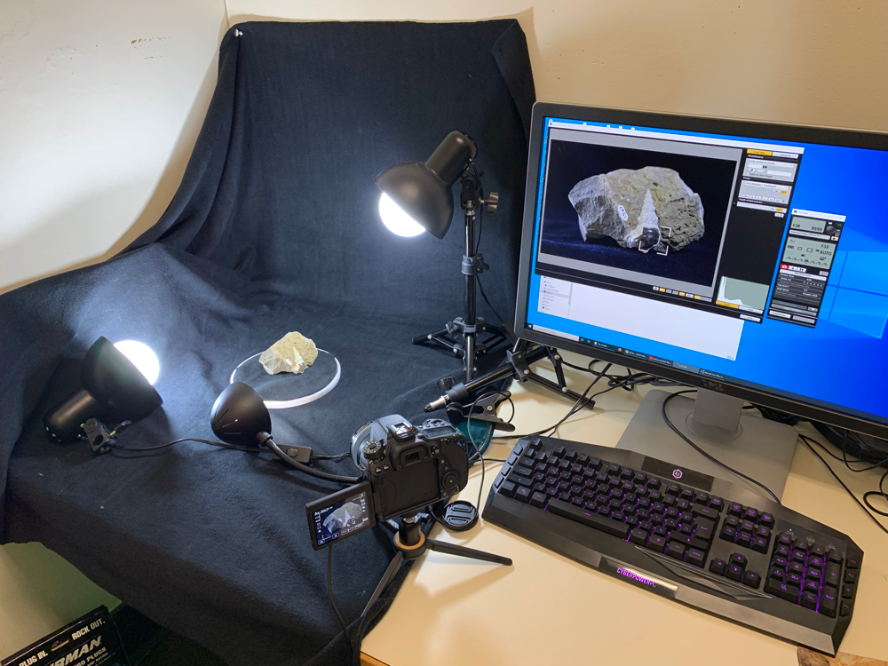
The photogrammetry workspace at the Paleontological Research Institution.

Step 1: Orient the lights around the specimen so that it is illuminated on all sides visible to the camera in order to minimize shadows (be prepared to move the lights for each individual specimen). We use two standing desk lamps as well as a clamp desk lamp for this purpose (see specifications above).

Step 2 (will vary depending on your camera; instructions are for a Canon 80D): Plug Micro-USB cord into computer and camera and then open ‘Remote Shooting’ on the EOS Utility program. Next, click ‘Live View shoot’ and then align the specimen so that the it fills the view as much as possible. Place the specimen in the center of the turntable and then focus the camera on the specimen. Finally, select ‘Depth-of-field preview’ - this allows more of the specimen to be in focus in the 'Live View' mode. In most cases, the camera was set to AV mode, had an aperture setting of F32, ISO was set to AUTO, and Image Quality was set to L 6000 x 4000 px jpegs.

Step 3: Take a photo of the specimen approximately every 10 degrees of rotation (degree markings were added to the turntable for convenience and consistency; see photograph below). Be sure to check that the specimen stays in view as it is rotated on the turntable (it is a good idea to test this in 'Live View' mode before you actually start capturing images). Adjust the lights as needed; note that there is also an exposure control on the EOS Utility program.

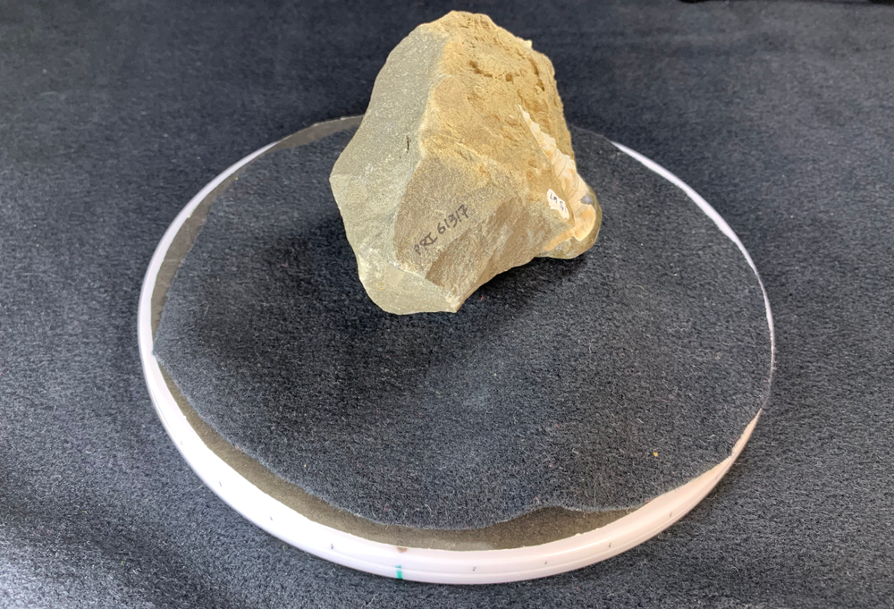
An inexpensive lazy susan with 36 10-degree markings added (blue mark indicates origin).

Step 4: Once finished with the first round of photos, rotate the specimen and repeat the process. Do this for 3-4 different angles, or until all angles/surfaces of the specimen have been photographed in more than one orientation.

Tips:

• A shallow box (e.g., a museum specimen box) filled with sand can be used for balance, whether that be sticking the specimen directly into the sand or leaning it against the box. In some cases, the box of sand can be covered with some black cloth to minimize the need for masking (see later steps). If the specimen must be stuck into sand for better balance, be sure to photograph the parts of the specimen that were in the sand when you capture another angle. It is best to start with the entirety of the specimen showing in the first set of photos and then target specific parts of the specimen in later angles.
• For flat slab specimens (example), the first set of photos should capture the specimen standing straight up. Cloth may be used to balance it, if necessary. For the second angle of photography, place it flat. If it is leaned against a box of sand, make sure to flip the specimen to photograph the back as well.
• If you are working with a wobbly specimen, some sand can be poured onto the turntable to diminish the movement.
• The number of total photos captured of each specimen will depend on the nature of each individual specimen. Typically, they should range between 108–216, which is between 3–6 different angles (36 photos per angle).

Part 2: Model Development in Agisoft

Overview of Agisoft Photoscan (Standard Edition)

When you create a new Photoscan file, five program components become available.

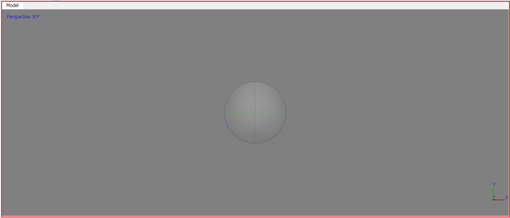
Model Perspective: This is where the model can be viewed and edited during the photogrammetry process. The sphere in the center can be used to center the model; this also shows you that you are in navigation mode. The red, green, and blue lines are the x, y, and z axes (respectively) of the model and can be used to rotate the model in a one direction if a single axis is selected.

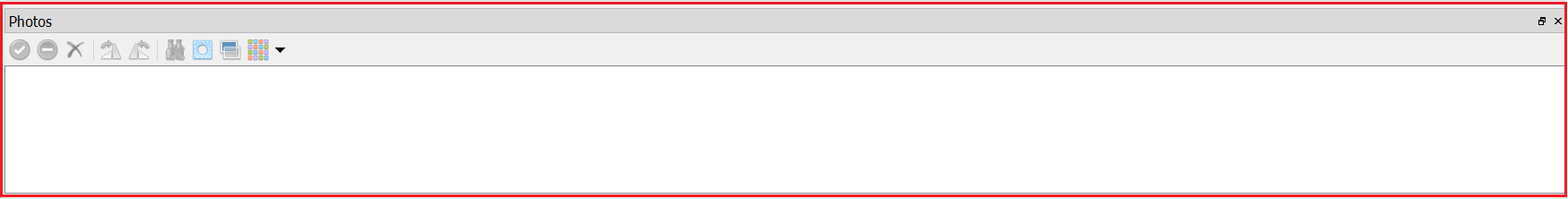
Photos: This is where the individual images of the specimen can be accessed and masks (see below) can be viewed. Cameras (=individual images) are denoted by the green check marks in the upper right of the image.

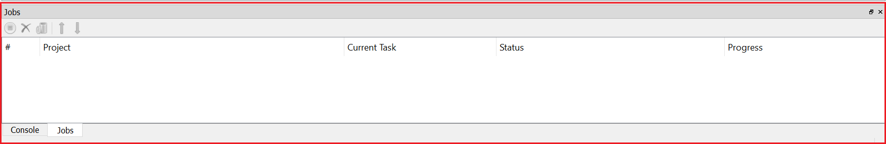
Jobs: This shows the progress for each task during model building.

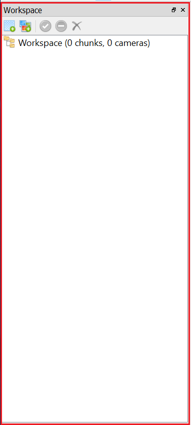
Workspace: The workspace component shows where the chunk(s) are managed. Chunks are groups of photos that will be used for construction of the model. Cameras are the individual photos within the chunks. Once the photos have been aligned, there is a third count of ‘points’, which shows how many points have been matched between all of the photos (this number will vary depending on each project’s size).

Workspace options include:

• Add chunk: This creates a new chunk where the photos of the specimen will be added.
• Add photos: This allows images to be selected and added to the chunk.
• Enable items: This allows for selected items to be used for the alignment process.
• Disable items: This allows selected items to not be used during the alignment process.
• Remove items: Deletes selected items.

Toolbar: The toolbar component allows varied commands to be executed.

Options:

• New: Opens a new file.
• Open: Opens a saved file.
• Save: Saves file.
• Undo: Undoes last action.
• Redo: Redoes undid action.
• Navigation: This allows for control of the position and angle of the model.
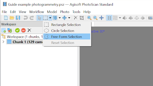
• Rectangle/Circle/Free-form Selection: This allows for the selection of specific points or mesh.
• Move region: This allows for the location of the region where the model is created to be moved.
• Move object: This allows for the location of the model in the region to be moved.
• Delete selection: Deletes selected points or mesh.
• Crop selection: Deletes non-selected points or mesh.
• Point cloud: View of original point cloud.
• Dense cloud: View of dense point cloud.
• Shaded: View of basic vertex colored mesh.
• Solid: View of solid colored mesh.
• Wireframe: View of wireframe mesh.
• Textured: View of final textured mesh.
• Show cameras: View of camera location and angle placement of photo alignment.
• Show aligned chunks: If there are multiple aligned chunks, this can be used to view them in the same model perspective.

Mouse controls and keyboard shortcuts:

• The mouse scroll wheel (if present) can be used to zoom in and out. It can also be clicked to move the model. This can help center the model in the Model Perspective.
• The space bar can be used to toggle between navigation and any selection tool.

Development of the Model

Uploading Photos

Step 1: Open a new Agisoft file (see above).

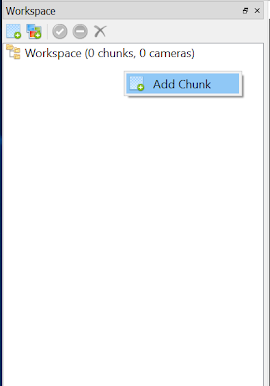
Step 2: In "Workspace," right click and select "Add chunk" from the drop bar. This will be called "Chunk 1."

Step 3: Right click on "Chunk 1." Hover over "Add" and then select "Add Photos."

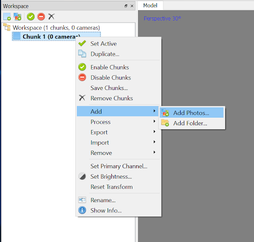
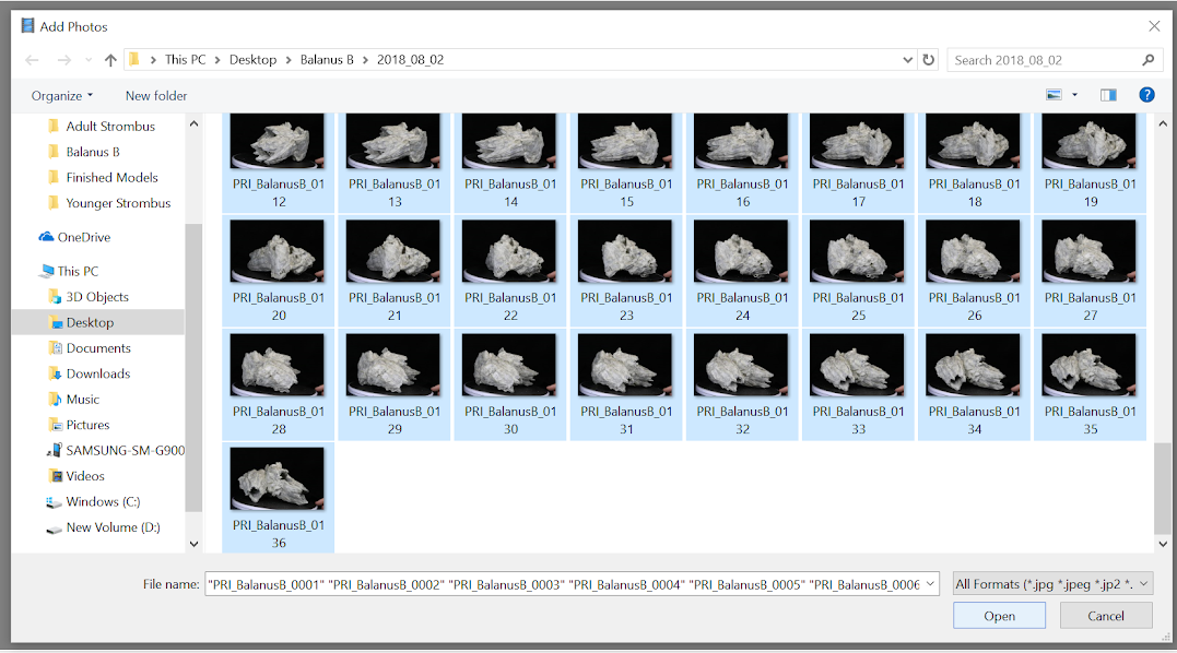
Step 4: Locate and select all desired photos of the specimen and then click "Open."

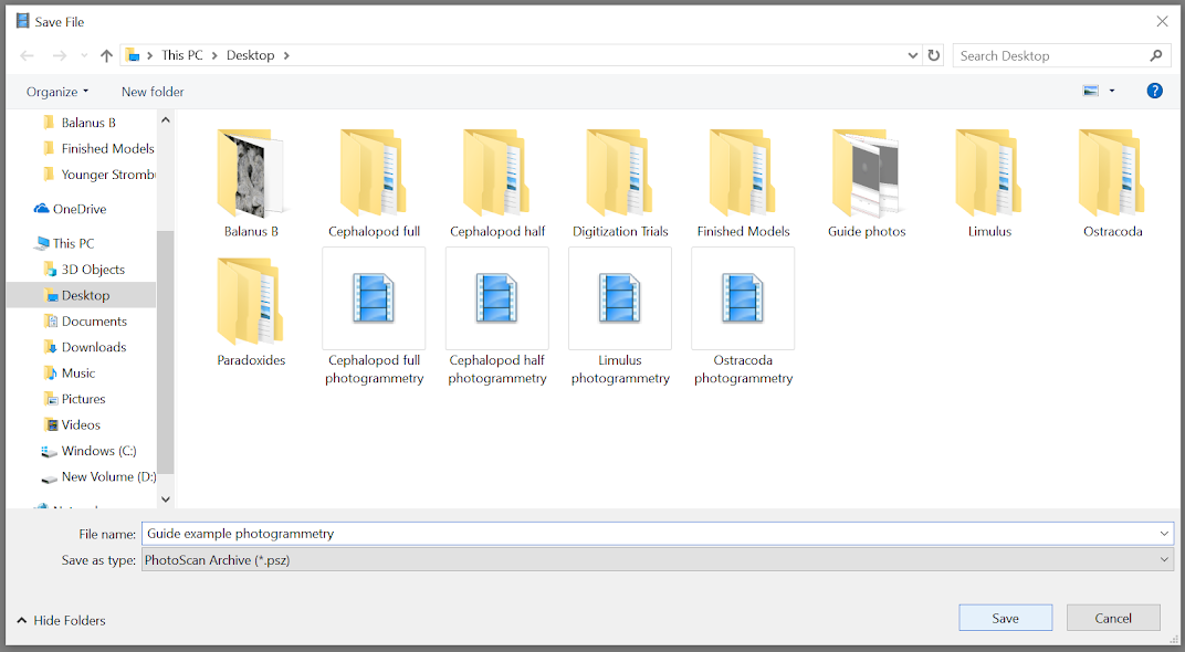
Step 5: Save the document as "*Specimen name*" photogrammetry."

Aligning Photos

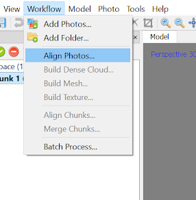
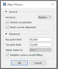
Step 1: From the toolbar, select "Workflow" and then "Align Photos..." (note that right-clicking the chunk in the workspace will also provide an "'Alight Photos..." option when the cursor is hovered over "Process"). This will open an option window that allows accuracies and point limits to be adjusted.

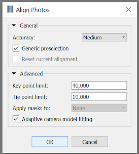
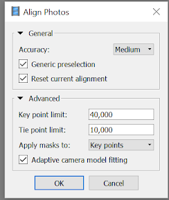
Step 2: This will open an option window that allows accuracies and point limits to be adjusted. Select "Medium" accuracy for alignment and set "Key point count" to 40,000 and "Tie point limit" to 10,000. After these are set, click "Ok."

This step may take some time to finish; it is a good time to photograph your next specimen or to work on developing other specimen models. Once this step is finished, be sure to SAVE!

Step 3: Once the "Align Photos" operation is complete, analyze the camera angles/locations by selecting the camera icon in the toolbar. Select the cursor icon in the toolbar to allow the model to be rotated with your mouse.

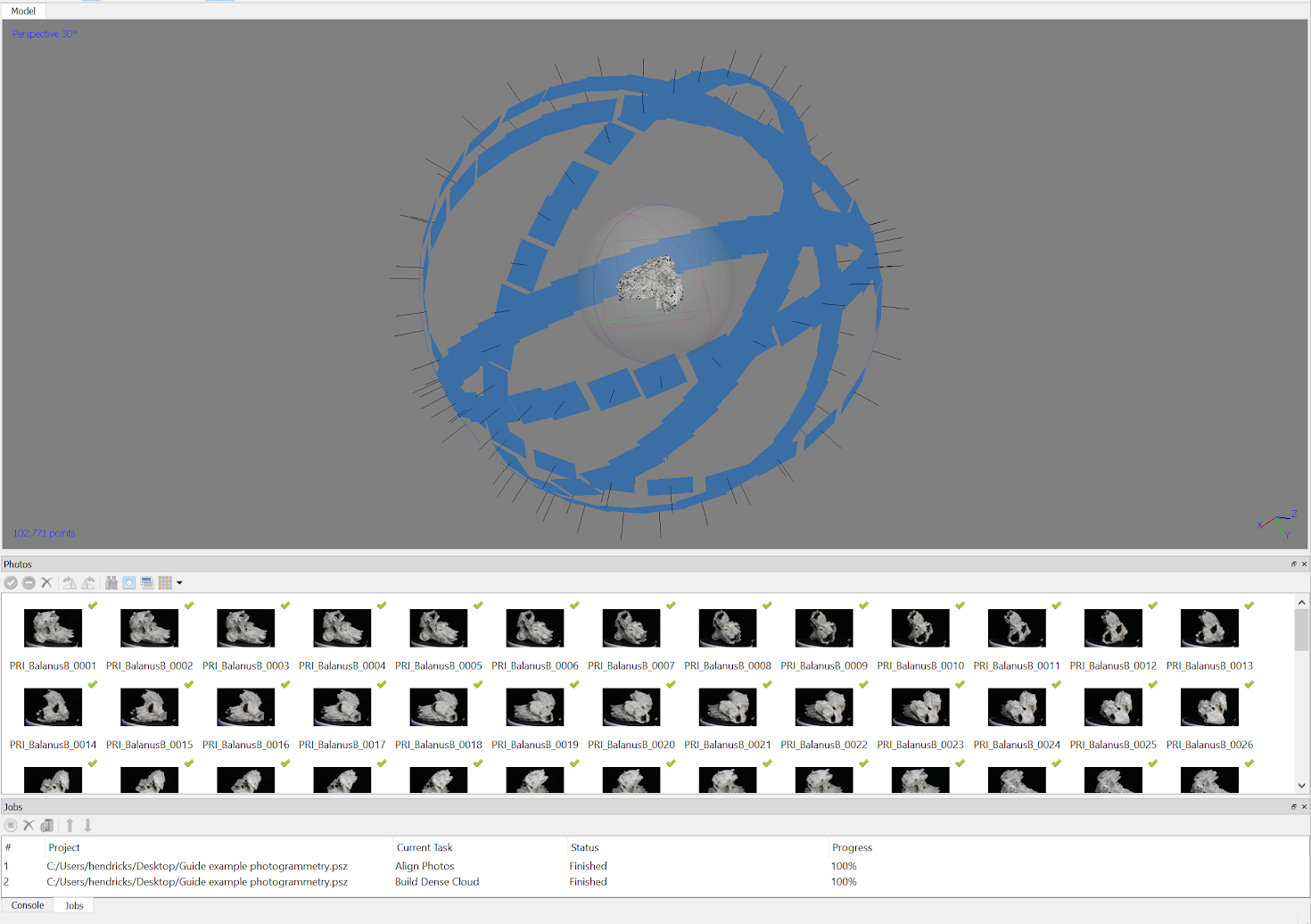
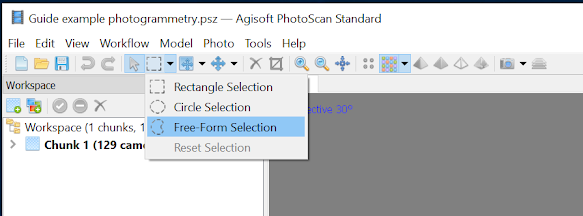
If the model and camera angles look correct, select the "Free-form" selection tool in the toolbar and remove any excess distal points that do not belong to the model.

This is done by clicking and dragging the cursor to select an area of points. The highlighted area and points selected will turn red. To remove them, click the "delete" key on the keyboard.

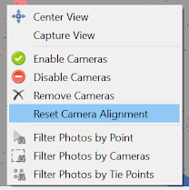
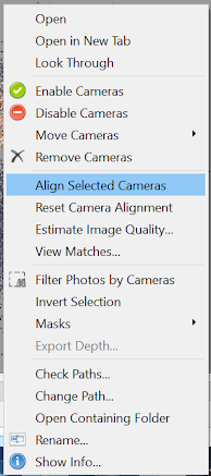
If the camera angles and/or basic model does not seem correct (e.g., the model has no distinct shape or there are blue photo locations stacked on top of each other), use the "Free-from" selection tool to highlight the incorrectly aligned images. Then, right click and select "Reset Camera Alignment.”

Next, in the Photos window, right click on one of the selected photos and click "Align Selected Cameras."

If the images positions do not become correct after realignment of the selected photos, then run the entire photo alignment again at either High, Medium, or Low accuracies. The program will run and match different points together each time the photo alignment is redone. Make sure to select "reset current alignment" in Photo alignment options window.

If running the photo alignment multiple times does not work and the points will not align on their own, then each image will have to be masked individually to narrow the point selection for the alignment. If this is the case, follow the instructions below for "Masking an Image."

Masking an Image

Note: You may skip these steps and continue to the "Building Dense Cloud" section if the camera locations and basic point cloud model are aligned correctly.

Step 1: In the "Photos" section, double click the first image labeled *Specimen name_0001*. In the toolbar, select the ‘Intelligent scissors’ (the lasso icon in the selection tools drop box) or press the ‘L’ letter key.

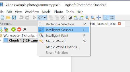
The "Intelligent Scissors" tool creates a continuous line to select irregular shaped areas. For this step, the goal is to mask the majority of the background. Unlike the "Free-form Selection" tool, this selection tool works by placing individual points around the specimen by clicking, not by dragging.

Make sure to follow the edge as closely as possible, but be careful that none of the actual specimen is masked, unless there is an unavoidable shadow (shadows can be cropped as well). To end the "Intelligent Selection" line, place a finishing point where the first initial point was placed.

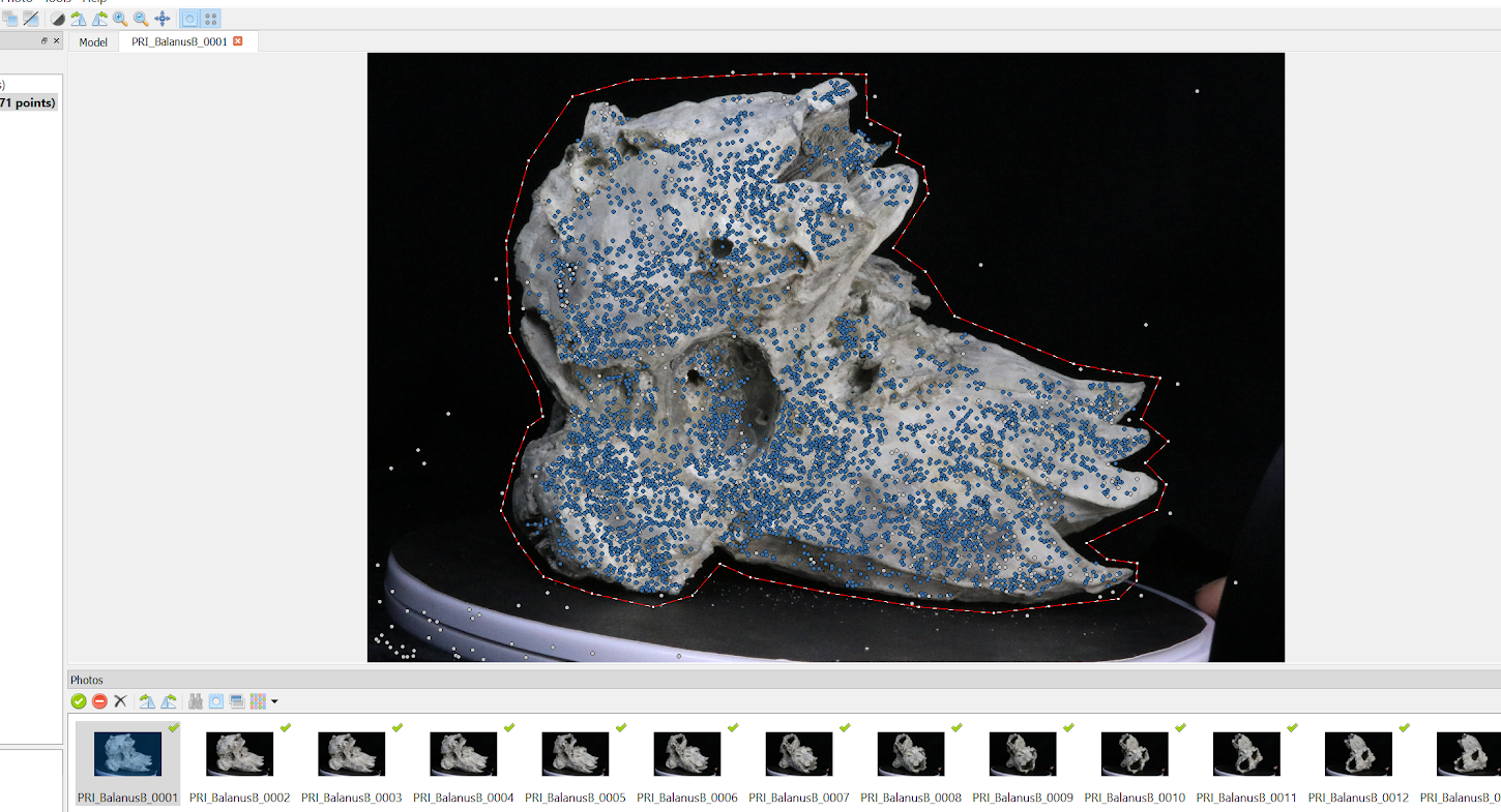
Since we want to mask the background and not the specimen itself, we need to invert our selection, which can be done by right clicking and selecting "Invert Selection."

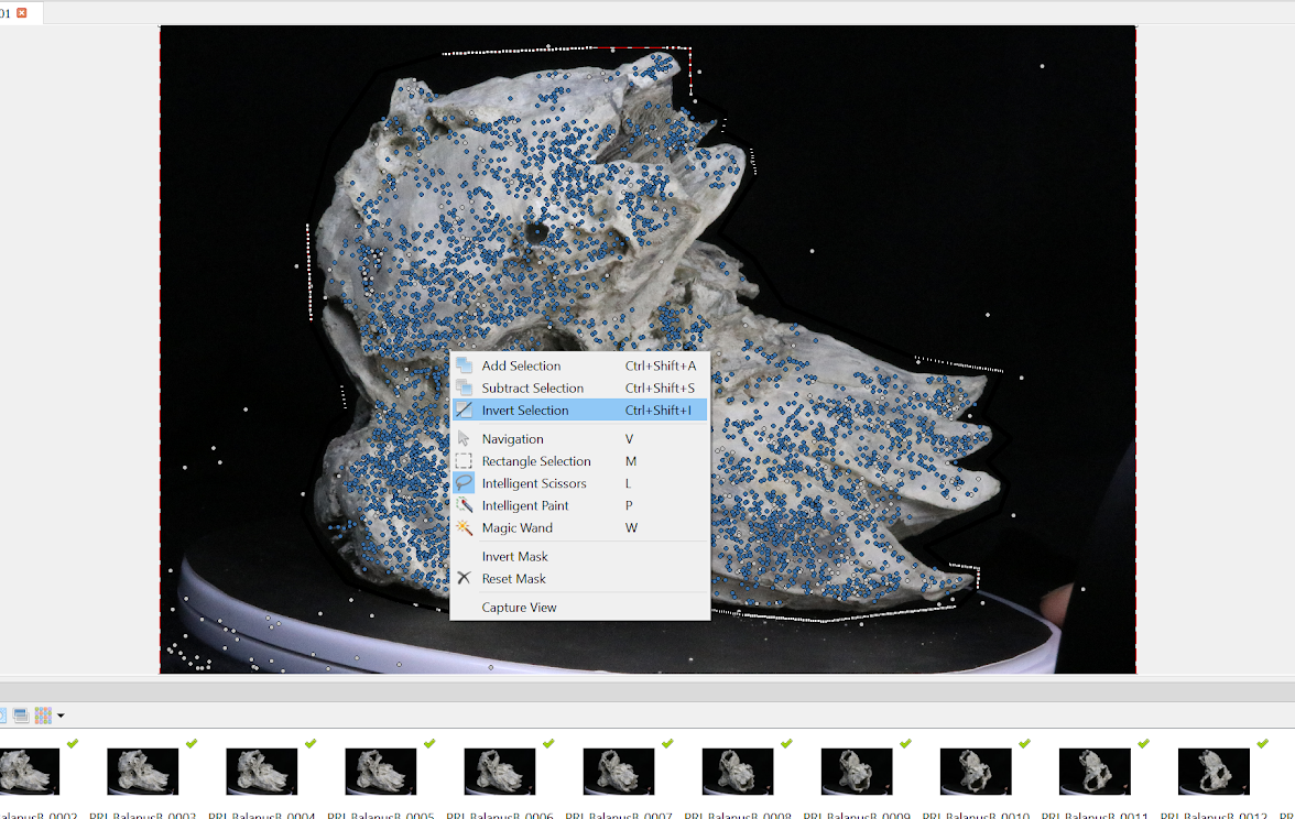
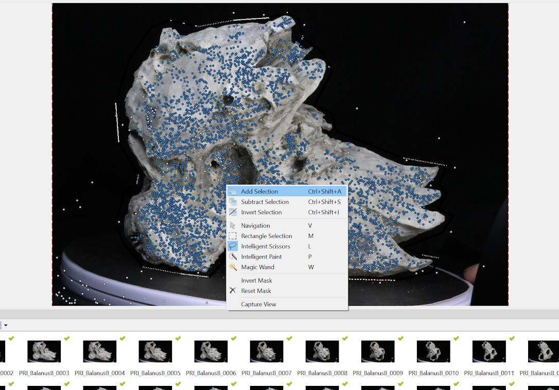
Then right clicking again, select "Add Selection."

Repeat this process until each image is masked. Remember to save continually throughout the masking process.

Step 2: Once all images are masked, return to the photo alignment process by opening the "Align Photos" window. Select "Advanced" and then select the option "Apply mask to: Key points." Then, click "Ok."

Building the Dense Cloud

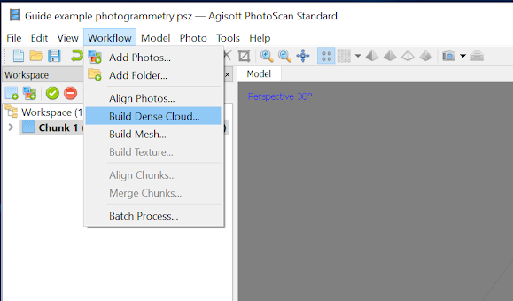
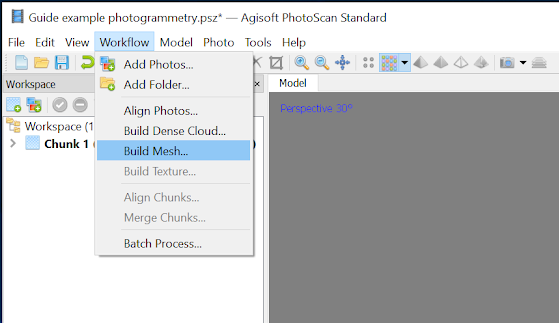
Step 1: In the toolbar, click "Workflow" and then "Build Dense Cloud…."

The "Build Dense Cloud" window will open. This window presents several options, including the quality at which the dense cloud is created.

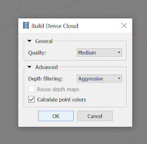
There can be some variance with this selection, but typically ‘Medium’ will give decent results without taking drastically more time. If the initial model from the photo alignment is sparse, run the dense cloud at a higher quality to give you more points. Click "OK" after you have made your selections.

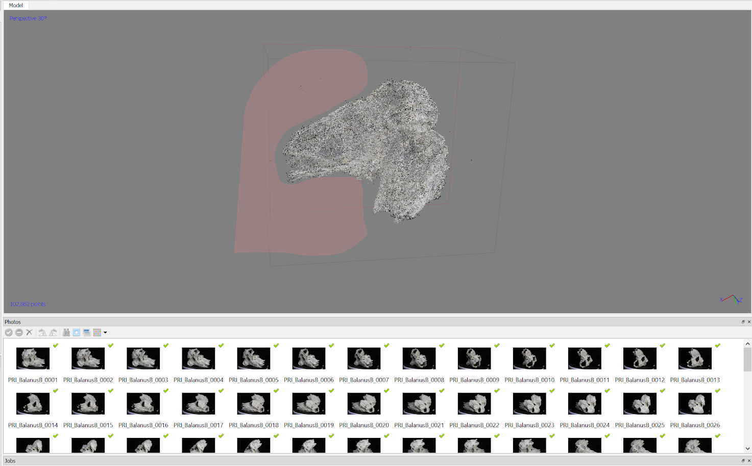
Step 2: To view the dense cloud model, select the "Dense Cloud" icon along the toolbar (the icon with sixteen multicolored dots). If the dense cloud model looks correct, select the "Free-form" selection tool in the toolbar and remove any excess distal points that do not belong to the model.

This is done by clicking and dragging the cursor to select an area of points. The highlighted area and points selected will turn red. This is the same cleanup process as the photo alignment process, but this model can be cleaned up more intensely to remove any excess points.

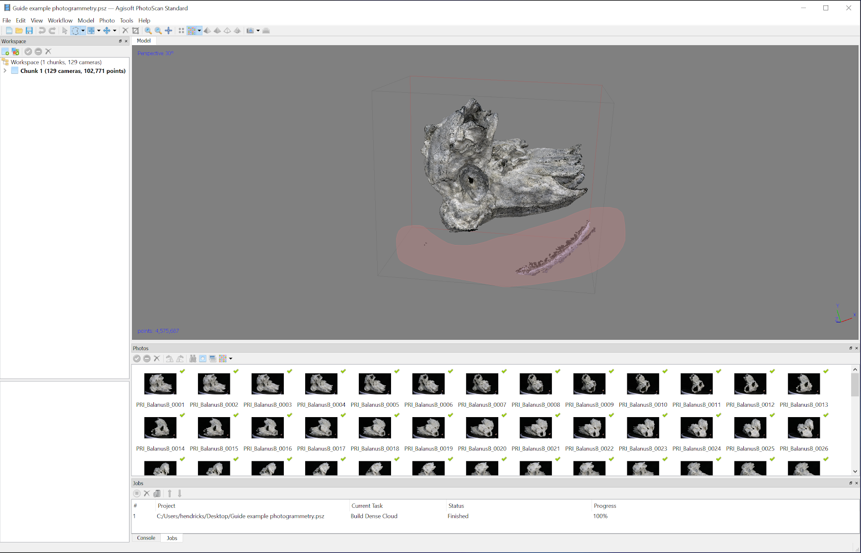
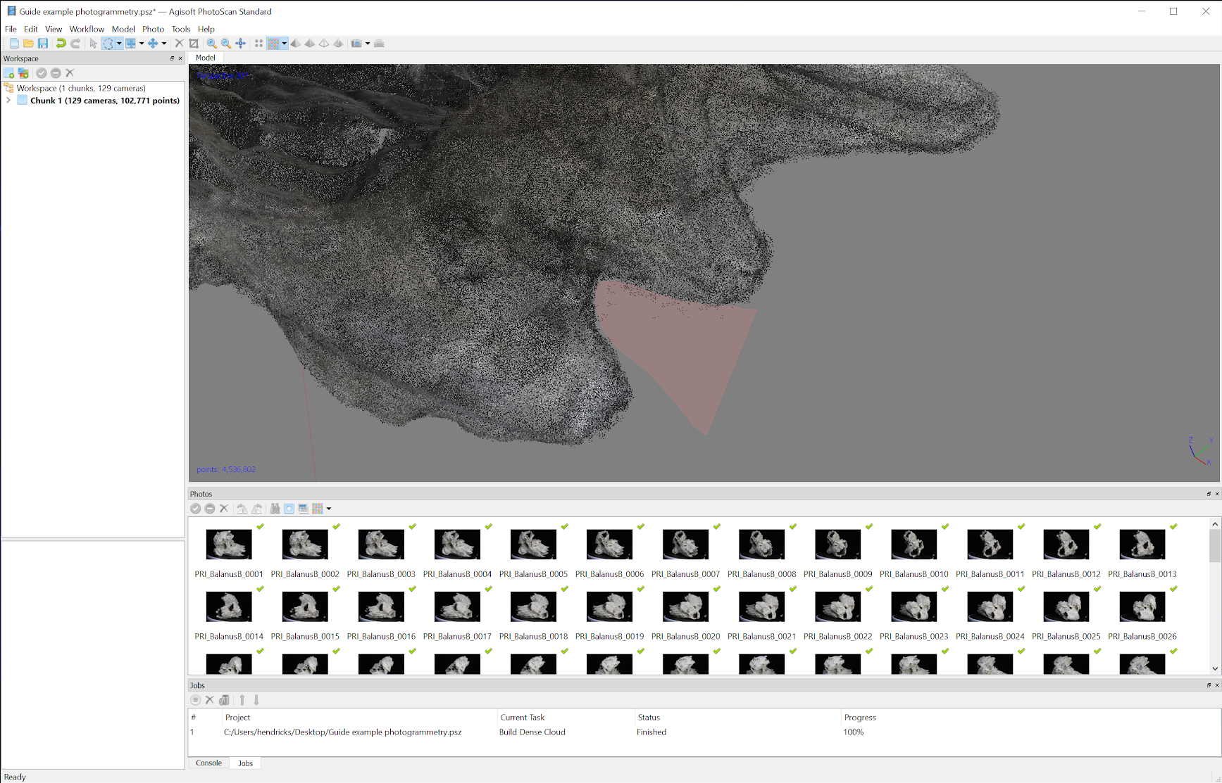
Make sure to save once you are finished with making your edits.

Building the Mesh

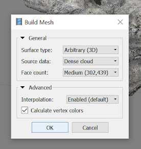
Step 1: In the toolbar, click "Workflow" and then "Build Mesh…."

The "Build Mesh" window will open. Set "Face count" to "Medium." Next, click "OK."

Step 2: Once the mesh is finished, select the left-most yellow and green pyramid icon on the toolbar to view the mesh model.

**Note: The user will determine what additional mesh editing changes to make in order to produce the best possible model. The importance of the following comments will depend on individual models.

During the mesh processing step, there might be excess dense cloud points that were transferred into the mesh model as floating blobs. These can be deleted with the "Free-form" selection tool in the toolbar (same tool from the photo alignment and dense cloud editing steps; see above).

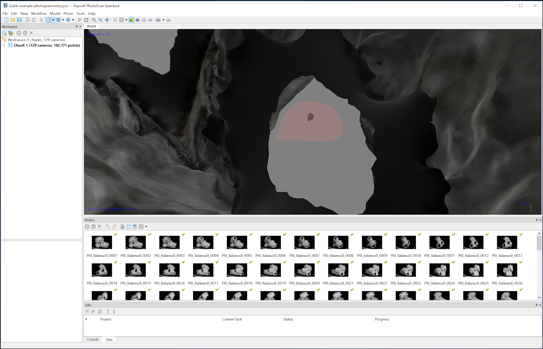
** Note that the image above was taken from within the mesh of model because the free-form selection tool will select mesh on all planes of the model if facing into the model.

If there is an edge or surface with a bit of mesh that is undesired, use the "Free-form" selection tool to highlight and delete the area. The edges should be smoothed slightly and then the hole(s) should be closed (see below). It is easier to close all holes at once after all undesired mesh has been removed from the model.

If there are significant errors in the model, consider restarting with a new alignment or the addition of another angle of images that encompasses the troublesome area, especially if the errors cannot be fixed with deleting or smoothing the problem area.

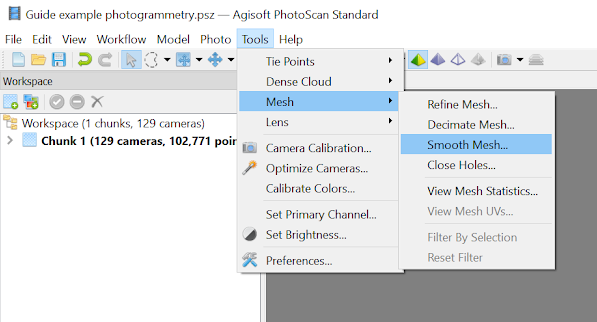
Step 3: The next step is to smooth the mesh. Before you begin, make sure to SAVE your model. Then, on the toolbar, select "Tools," "Mesh," and then "Smooth Mesh...."

It is the user's preference as to the amount of smoothing to apply. Levels 1–3 are minimal change, 4–5 are more noticeable change, 6–9 very noticeable change, and  >10 drastic change.

Note that a specific area of the model can be selected with the "Free-form" selection tool to be smoothed separately from the rest of the model. This is done by selecting "Apply to selected faces" in the "Smooth Mesh" option window.

Importantly, there is no undo option for smoothing. So, it is wise to first smooth less than is needed and repeat only if needed. (Again, make sure to save model before beginning the smoothing process!)

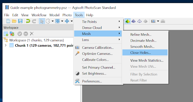
Step 4: The final step of mesh building is to close any holes that might exist. On the toolbar, select "Tools," "Mesh," and then "Close holes...."

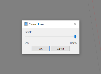
In order to close most holes, set the "Level" in the "Close Holes" window to 100%.

Some edges of the closed holes will not match exactly with the rest of the mesh. This could possibly be fixed by smoothing the entire mesh slightly. If not, remove the closed holes (this can be done by using the undo button in the toolbar, or CRTL+Z) and either remove more of the surrounding mesh of the undesired area, or try to smooth the original mesh to a desired shape.

If there is a problem area of the model that is too rough to smooth, the entire area can be deleted and then closed. Be aware this will possibly change the shape of that area if it is on a corner or distinct feature of the model. Flatter surfaces work best for this option.

Building Texture

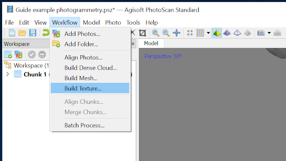
Step 1: On the toolbar, select "Workflow" and then "Build Texture…."

The "Build Texture" window will open. Set "Mapping mode" to "Generic."

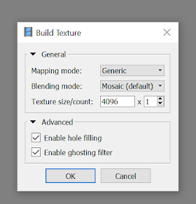
Note that there is limited editing that can be done to the texture itself.

Step 2: Once the texture is finished, select the right-most pyramid icon (with the sky and tree) on the toolbar to view the model with texture.

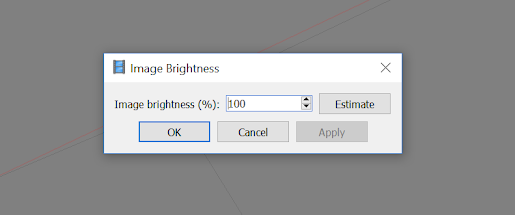
If the overall exposure of the model is too bright or too dark, select "Tools" from the toolbar, then "Set Brightness...."

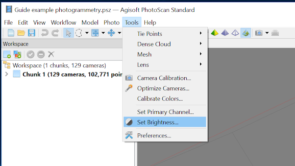
Lower the percentage if the model is too bright; raise the percentage if it is too dark.

Step 3: If there is a section or edge of the model that is black, return to the mesh model and try to find and remove the area and then build the texture again. If that does not fix the area, assess the overall model and determine if the dark area significantly diminishes its quality. Minor dark areas may be  diminished on Sketchfab after posting (see Part 3 below).

If dark areas do significantly diminish the overall quality of the model, taking another round of photos that better capture the troublesome area may fix this problem, as may masking these areas. These photos will need to be added into the original chunk and the process will then need to be repeated from the beginning.

Exporting the Model

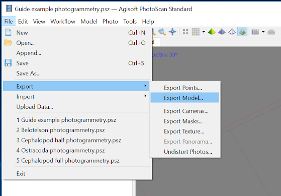
On the toolbar, select "File," "Export," and then "Export Model...."

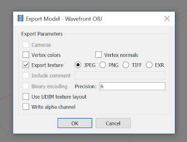
Select the folder of choice and then save the file with a sensible name. The file type should be set to .obj. Additionally, deselect "Vertex colors" and export the texture as a .jpeg. Click "OK" to complete the exporting process.

Part 3: Publishing to Sketchfab

Just as Youtube is a platform for sharing videos online, Sketchfab (sketchfab.org) is a platform for sharing 3D models (either scanned or created using photogrammetry).

You will need to create an account on Sketchfab in order to upload models. The instructions below pertain to a "Pro" level account (options available will depend on the account level that you choose).

Step 1: The first step is to upload your files to Sketchfab.

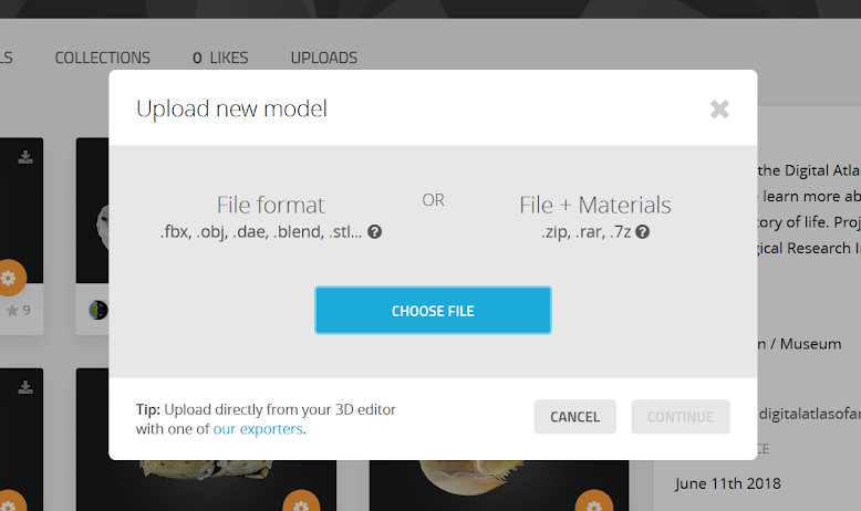
Select "Upload" (blue bottom at upper right).

After the "Upload new model" window opens, select "Choose File."

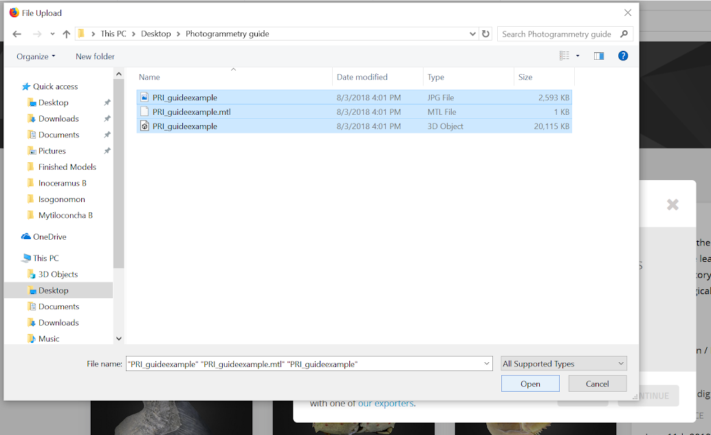
Select the desired files for the model that you wish to upload. These should include a .jpeg file, an MLT file, and a 3D object file (.obj). Navigate to these. After they are selected, click "Open." The files will then be uploaded to Sketchfab.

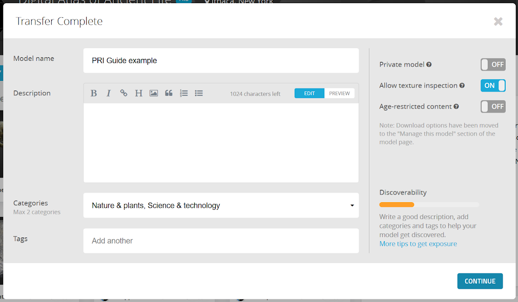
Step 2: Once the model is uploaded, select "Properties." This allows options to assign the model a name and add pertinent descriptive information, categorical information (for fossils we typically select "Nature & Plants" and "Science & Technology"), and add tags that best apply to the specimen. Adding this information makes the model more discoverable when users search the Sketchfab site.

Step 3: If you wish to make your specimen free to download and to have Creative Commons licensing, select the corresponding options.

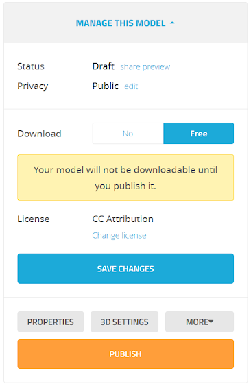
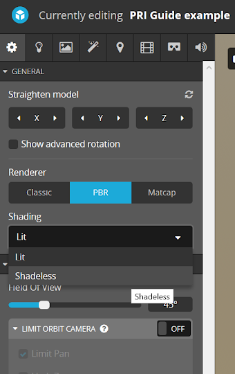
Step 4: It is possible to change the appearance of your model by using options that become available by selecting "3D settings."

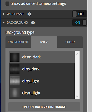
We typically set "Shading" to "Shadeless" under the "General" menu. We also typically use a "Clean Dark" background under the "Background Type" dropdown menu.

Step 6: If the position of the 3D model needs to be changed, select "Show advanced rotation" (within the "3D settings" interface). Adjust as necessary.

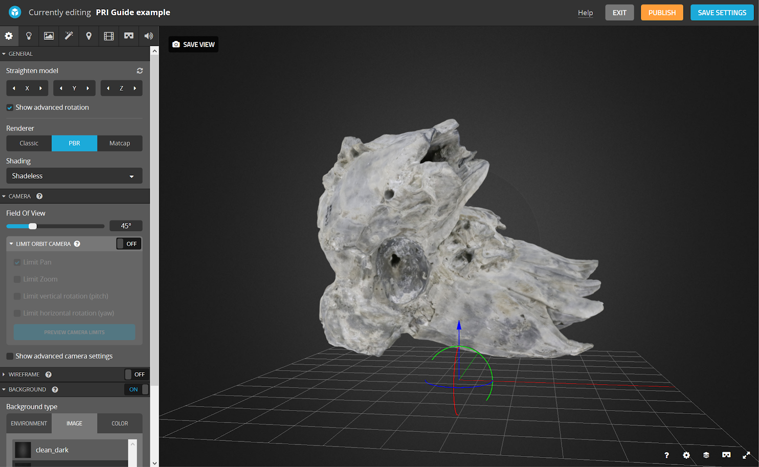
If the camera view needs to be limited, turn "Limit Orbit Camera" to "On" and either select "Limit vertical rotation" or "Limit horizontal rotation." Limiting the pan will not allow the model to be moved from the original z-axis.

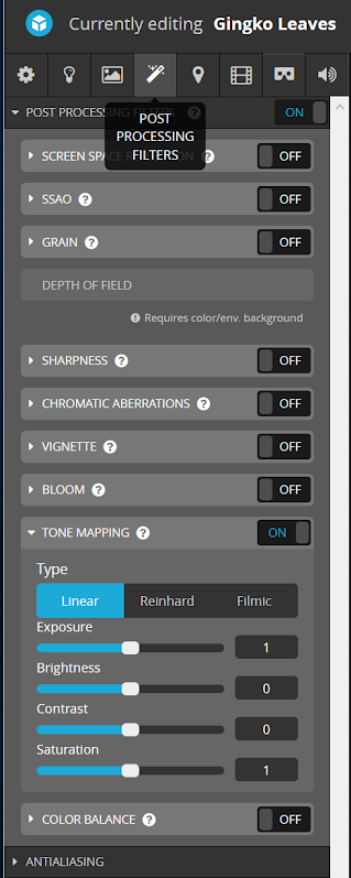
Step 7: If the texture has minor color corrections that need to be made, these can be changed using the functions available under "Post Processing Filters" (also available under "3D Settings"). Exposure, brightness, contrast, and saturation of the texture can all be altered according to user preference. Contrast, in particular, can be used to diminish the intensity of dark-shaded areas.

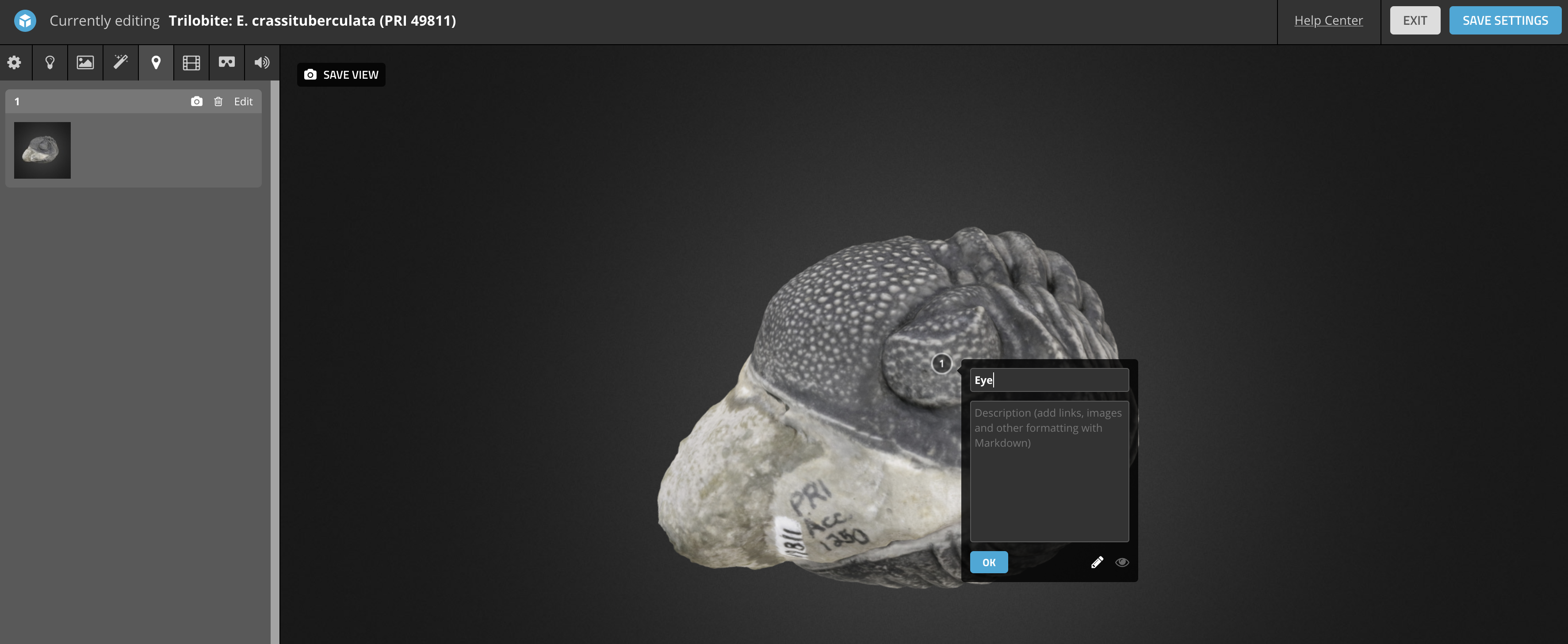
Step 8: If desired, it is possible to annotate features of interest on the model by selecting the upsidedown tear-drop shaped icon available in "3D Settings."

Step 9: Once you have modified the appearance of the model to your satisfaction using the tools availalbe in "3D Settings" (there are many more than those briefly mentioned here), click "Save View" (blue button in upper right corner). Once this is finished, "Publish" can be selected. The model’s web page will load and the finished and published model will be able to be viewed. Note that it is possible to change the model's properties and 3D settings at any time after publication.

Your 3D model is now ready to share with the world. Congratulations!!