

Chapter contents:
Paleoecology
– 1. Paleoenvironmental Reconstruction
– 2. Biogeochemical Analysis and Paleoecology ←
– 3. Predation in Paleoecology
–– 3.1 Insect Herbivory in the Fossil Record
–– 3.2 Drilling Predation in the Fossil Record
–– 3.3 Dinosaur Predation in the Fossil Record
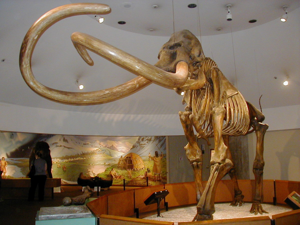
Above image by WolfmanSF; Creative Commons Attribution-Share Alike 3.0 Unported license.
Overview
Fossils have the potential to provide a wealth of information about the environment in which organisms were living. In this section, which is closely related to the preceding Paleoenvironmental Reconstruction section, we will take a closer look at the information harbored inside of the fossils themselves. The extraction and application of this information requires an understanding of biogeochemistry, which is the study of the integrated biological, geological, and chemical processes (e.g., water and carbon cycles) and reactions that dictate the dynamics of natural environments. As organisms live and grow, they incorporate isotopes—atoms containing a greater or lesser number of neutrons than typically found in an atom of the element—of oxygen, carbon, and nitrogen into their skeletal hard parts. There are many different isotopes and they fall into two general categories: radioactive and stable. Radioactive isotopes decay over time (e.g., uranium-238 eventually turns into lead-206) and are often used to find absolute ages of rocks, minerals, and fossils (An introduction to dating with isotopes can be found in the Geological Time chapter). In this section, we will look more closely at stable isotopes, which do not naturally change on their own as the radioactive isotopes do. Studies of stable isotopes can reveal detailed information about growth rates, life spans, seasonality, environmental conditions, and even evolution of the earliest life on earth.
Oxygen isotopes
Although isotopes of a variety of elements can be assessed, oxygen (O) and carbon (C) isotopes are among the most commonly studied. In large part, this is because they are common in the environments where organisms live and are readily incorporated into biological tissues. Two isotopes of oxygen, and the ratio between them, are commonly studied: 18O and 16O. Typically, an atom of oxygen contains eight neutrons in its nucleus along with eight protons; this is 16O. Occasionally, two extra neutrons are incorporated in the nucleus, creating 18O. A variety of other oxygen isotopes can occur; however, only 18O and 16O are commonly studied. As a consequence of the extra neutrons in its nucleus, 18O has a greater mass than 16O. When incorporated into a water molecule, this extra mass means that a water molecule with 18O is less likely to evaporate than a molecule composed of 16O, if all else is equal. Because of this, 18O tends to accumulate in oceans and 16O, as a part of a water molecule, is more likely to evaporate and return to Earth as freshwater precipitation. Thus, ocean water can be said to be “heavy” compared to freshwater.
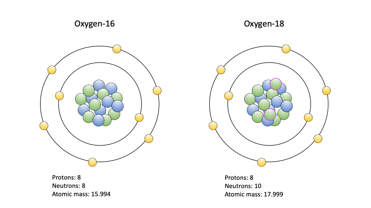
The two oxygen isotopes commonly used in paleoecological studies: 16O (left) and 18O (right). Protons are blue; neutrons are green, with a purple outline indicating an extra pair in the 18O isotope nucleus; electrons are yellow. Figure by Jansen Smith.
There are several biologically important outcomes of this difference between isotopic water compositions. In general, the oxygen atoms making up molecules in an organism tend to reflect the types of isotopes in the organism’s environment. This means that by examining the proportion of 18O and 16O in a fossil (or living) organism, we can determine whether it lived in a freshwater or oceanic environment. The ratio of 18O:16O is typically converted to a δ18O value, which can be thought of as enrichment (more positive values) or depletion (more negative values) of 18O as compared to a standardized value. The standardized value, for example the average 18O:16O of seawater, allows scientists to compare different δ18O values to each other when studies take place in different locations and times.
In studies using oxygen isotopes it is important to understand other reasons why concentrations may vary, namely due to variations in temperature. Water molecules containing the lighter isotope, 16O, tend to evaporate more easily, meaning most precipitation is depleted in 18O. Consequently, 16O is more likely to turn into ice during periods when the Earth is cold and remain trapped in glaciers, ice sheets, and ice caps. During these colder times, organisms typically show higher 18O concentrations because the heavier isotope is more readily available in the environment. The opposite is also true. During warmer periods, there is less ice on Earth and therefore more 16O available to organisms for their use. Because the concentrations of 18O and 16O can change due to multiple factors (e.g., habitat, seasonality, climate change, organismal metabolism), it is important to have a some understanding of these potentially complicating factors prior to drawing conclusions based on isotopic data.
As is also the case with carbon, the manner in which plants use the different oxygen isotopes can influence the δ18O values found in animal fossils. Relating to oxygen, this difference is largely controlled by evapotranspiration—the sum of water vaper entering the atmosphere via evaporation and transpiration. When humidity is low and temperature is high, the rate of evapotranspiration will be relatively high (assuming all else is constant). Thinking about the mass of 18O and 16O atoms, how should the ratio of 18O:16O compare at high and low evapotranspiration?
In this short video, you can watch a schematic representation of evapotranspiration. After the rain falls, it soaks into the ground and, eventually, the plants absorb some of the water. When the sun reappears temperatures rise, water is evaporated out of the ground. The plants also lose water from their tissues through the process of transpiration. Together, these processes are referred to as evapotransportation. "Understanding Evapotranspiration (ET)" by webekeit. Source: YouTube.
Because 16O is lighter, it will compose a large percentage of the oxygen atoms lost through evapotranspiration and the plant would be “enriched” in 18O as a result. On a warm summer day, evapotranspiration will be high, as will the δ18O value of the plant. An herbivore eating the plant on the warm summer day will then also likely exhibit a high δ18O value. To the contrary, an herbivore consuming plants during a cold winter, at night, or in an aquatic habitat will have a relatively low δ18O value because little evapotranspiration occurs at these places and times. This relationship is useful because it can help assess herbivore behaviors in the past. For example, imagine two co-occurring species (as indicated by their presence in a fossil assemblage) that have exactly the same diet, but one has a significantly lower δ18O value than the other. What might explain this difference? In this case, the species with the lower ratio likely did its eating during the night, when evapotranspiration was low and plants retained more of their 16O. If we knew that the two species were both herbivores but did not have the same diet, different life habits, like consuming aquatic plants or consuming terrestrial plants, could also explain the difference.
The ratio of oxygen and other isotopes can vary significantly both between individuals in a community and within an individual. These sources of variability, which have been affirmed in studies of living organisms, can be beneficial depending on the goals of a study. For example, variability within an individual can be a very good thing if you are interested in studying growth rate or lifespan. In this case, it would be important to use a body part that continues to grow throughout an organism's lifespan, such as an elephant tusk or a clam shell, and therefore continuously records environmental conditions. (Bone is not useful for this, unfortunately, because it is continuosly reworked.) As we saw above, δ18O values are heavily influenced by temperature and thus can be used to assess seasonal patterns, with δ18O increasing during colder intervals (when proportionately more 16O is locked away in ice) and decreasing during warmer intervals. Looking at the image below, how old do you think this clam was when it died?
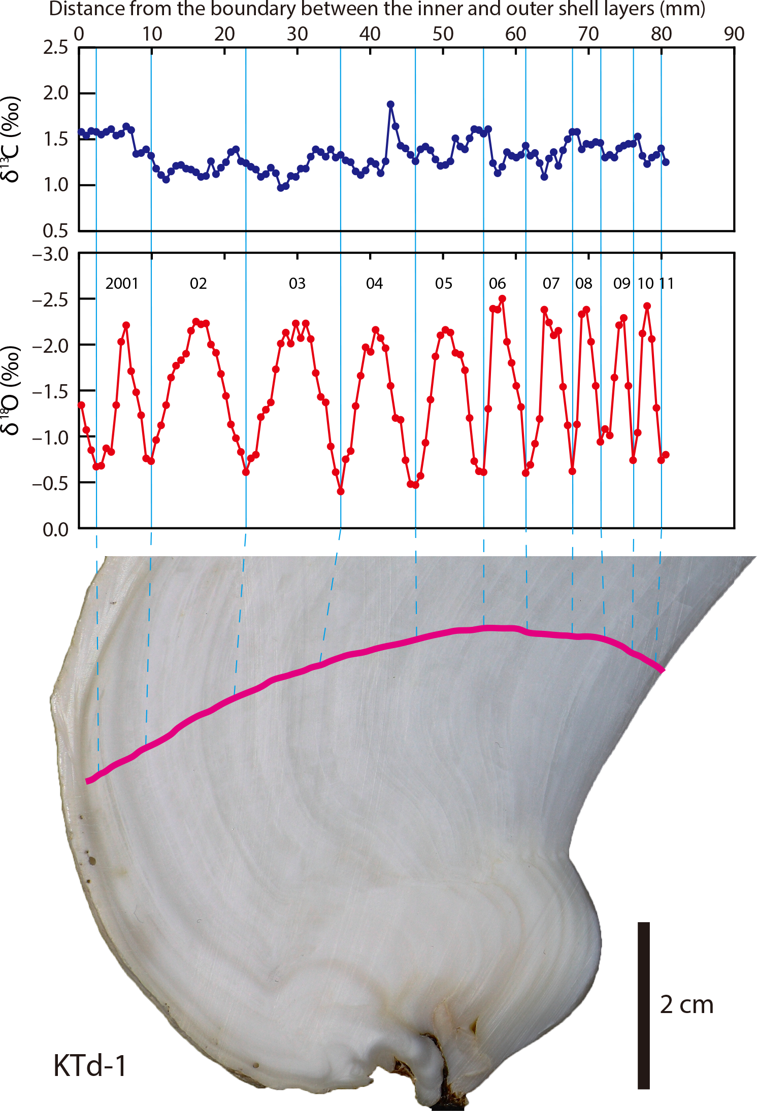
The top panel shows the carbon isotopes accumulated in the shell of the Tridacna clam. The middle panel shows the oxygen isotope profile, with each peak labelled for the year when the clam was alive. This clam was at least ten years old. The bottom image shows where the clam shell was sampled with a pink line. Notice that this pink line is perpendicular to the feint lines of the shell, which show grow within each year. Published caption: "δ13Cshell and δ18Oshell profiles of a Tridacna derasa shell (KTd-1).Pink line indicates the sampling transect." Figure from Yamanashi et al. (2016) in PLoS ONE; Creative Commons Attribution 4.0 International license.
As indicated by the ten peaks and valleys, this clam was likely at least ten years old when it died. (Note, though, that these data do not tell us how old the fossil actually is, only how long it lived.) By examining data like you just did, paleoecologists can get a better sense of how life span changes over time, if organisms change their rate of growth, or even season of death. Although it can be a complicating factor at times, within-individual variation can be highly informative.
Variability between individuals of a species can provide a more refined perspective on what was “normal” for the species. As with any group of individuals, there are likely to be subtle differences between them due to their genetics and the environments in which they live. Consequently, it is often a good idea to sample as many individuals as possible, though the cost of sample analysis can be prohibitive. In many ways, analyzing isotopic samples from multiple individuals is like having insurance against abnormalities. Though it might be unlikely, there is always a chance that, in assessing a single individual, you have selected an individual that was in some way abnormal, or its remains were unexpectedly altered by taphonomic processes. Analysis of multiple individuals presents an average for the population and gives a sense of the natural range of variability that existed in the population. This consideration is not limited to analysis with oxygen isotopes and, more broadly, can be extended to many scientific analyses.
Carbon isotopes
Like oxygen, there are many isotopes of carbon, but only two are commonly studied: 13C and 12C. The typical carbon atom, 12C, contains six neutrons and six protons, whereas 13C contains a seventh neutron. This extra neutron makes 13C slightly harder to use from a biological perspective. As a result, biological life forms, including the fossils they left behind, tend to have lower ratios of 13C:12C than their surrounding environment. Like the oxygen isotopes, this ratio is standardized and expressed as a δ13C value, where more positive values indicate a greater amount of 13C relative to 12C.
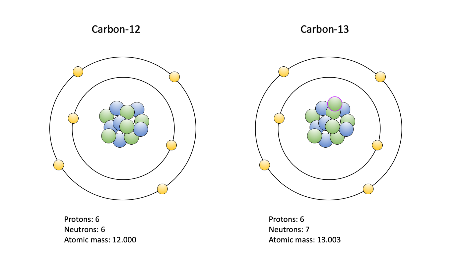
The two carbon isotopes commonly used in paleoecological studies: 12C (left) and 13C (right). Carbon-14 is also used, but primarly to date fossils; it is not depicted. Protons are blue; neutrons are green, with a purple outline indicating an extra in the 13C isotope nucleus; electrons are yellow. Figure by Jansen Smith.
The biological affinity for 12C rather than 13C has allowed scientists to identify some of the earliest life on Earth. As described in the video below, the earliest evidence of life on earth is in the form of low δ13C values, which we only find today in association with living organisms. Carbon with these ratios has been found in several places and indicates that life may have arisen on Earth 4.1 billion years ago.
"The Search for the Earliest Life" by PBS Eons. Source: YouTube.
Carbon isotopes can be used in a variety of ways, commonly including diet and paleoenvironmental reconstruction. Although organisms preferentially use 12C over 13C, not all organisms use them in the same ratio. For example, different groups of photosynthesizing plants (e.g., C3, C4 plants) use slightly different chemical pathways to convert carbon dioxide into sugars and oxygen, resulting in different ratios (watch the video below for an explanation of these differences). C3 plants, which includes most trees, shrubs, and cool climate grasses, produce lower δ13C values than C4 plants, which includes primarily the warm climate grasses. We can study living C3 and C4 plants and apply taxonomic uniformitarianism to translate this information in the past. Because the pathways used by C3 (Calvin cycle) and C4 (Hatch-Slack cycle) plants differs, when an animal consumes plants with different δ13C values, the animal maintains a similar ratio in their tissues (e.g., bone, tooth enamel). This means we can reasonably determine what types of plants the animal ate and, thereby, gain additional information about environment. Through analysis of the carbon isotopes and their preserved ratios in vertebrate fossils, as well as through comparisons with plants and animals living today, it’s possible to distinguish whether the community lived in a forest with a dense canopy or an open grassland.
"How C3, C4 and CAM Plants do Photosynthesis" by BOGObiology. Source: YouTube.
These carbon ratios can further explain the manner in which similar species—at least through appearance of their fossils—coexisted in the same community. Often δ13C values from different species reveal subtle differences in their primary plant food, demonstrating that, although there was competition between herbivorous animals, it did not prevent them from coexisting. Comparison of δ13C values for diet reconstruction can also be extended to identify carnivorous species. In large part, this differentiation is possible because of how carbon is used by different components of the body. Collagen—a protein abundant in connective tissues of vertebrates—only retains the carbon that is derived from proteins in an animal’s diet. Hydroxyapatite—commonly included in vertebrate bone and teeth—retains the carbon from the entire diet, which includes the fats, carbohydrates, and proteins consumed by the animal. Conveniently, fats, carbohydrates, and proteins exhibit different δ13C values, with fats having the lowest, carbohydrates having intermediate, and proteins having the highest δ13C values. In essence, the different usage of carbon means that the difference in the δ13C values between collagen and hydroxyapatite in the same animal will be greater for an herbivore than for a carnivore. Thus, by comparing δ13C values in a fossil community, it becomes possible to reconstruct the food web describing the species-species interactions in that community.
Other useful isotopes
When reconstructing food webs and trophic levels—levels are associated with organisms with similar functions and dietary requirements—it is common to use nitrogen isotopes alongside, or in place of, carbon isotopes. As with oxygen and carbon, nitrogen can exist as several different isotopes but only two, 15N and 14N, are commonly studied. A typical nitrogen atom, 14N, contains seven neutrons and seven protons in its nucleus. By comparison, 15N contains an extra neutron. Conveniently, δ15N values tends to increase by approximately 2–4% for each increase in trophic level (e.g., coyotes are at a higher trophic level than squirrels). Once again preserved in collagen, these differences in δ15N values provide critical information for reconstructing diets and interactions in the past.
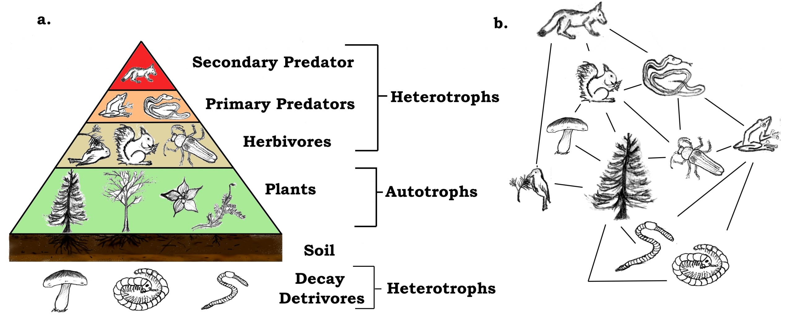
"A trophic pyramid (a) and a simplified community food web (b) illustrating ecological relations among creatures that are typical of a northern Boreal terrestrial ecosystem. The trophic pyramid roughly represents the biomass (usually measured as total dry-weight) at each level. Plants generally have the greatest biomass. Names of trophic categories are shown to the right of the pyramid. Some ecosystems, such as many wetlands, do not organize as a strict pyramid, because aquatic plants are not as productive as long-lived terrestrial plants such as trees. Ecological trophic pyramids are typically one of three kinds: 1) pyramid of numbers, 2) pyramid of biomass, or 3) pyramid of energy." Figure and caption by Thompsma; Creative Commons Attribution 3.0 Unported license.
If attempting to reconstruction past habitat use of an organism or species, strontium isotopes are a good choice. Strontium, as 87Sr and 86Sr in this context, is ingested through the food and water an organism consumes and becomes a part of its tooth enamel. Unlike the isotopes covered so far, 87Sr is a radiogenic isotope, meaning that it is formed through the radioactive decay of another isotope, rubidium (Rb) in this case. Over time, 87Rb decays to 87Sr, which is compared to 86Sr. Differences in the strontium isotope ratio (87Sr:86Sr) are due to differences in the underlying geology in the region where the animal lived. This means that when an animal moves from one geologically distinct area to another it will incorporate a different 87Sr:86Sr ratio from each area. The 87Sr:86Sr ratio is highly dependent on the original type of rock in the area and also on how old the rocks are. Older rocks have a higher 87Sr:86Sr ratio because there has been more time for 87Rb to turn into 87Sr. Thus, when applying strontium isotopes to understand habitat use and movement (e.g., migration), it is helpful to understand the underlying geology of the region at the time the organisms were living to help interpret the data. This approach is commonly applied to the study of early hominins (our early evolutionary cousins) in addition to studying movement and habitat use patterns of other mammals.
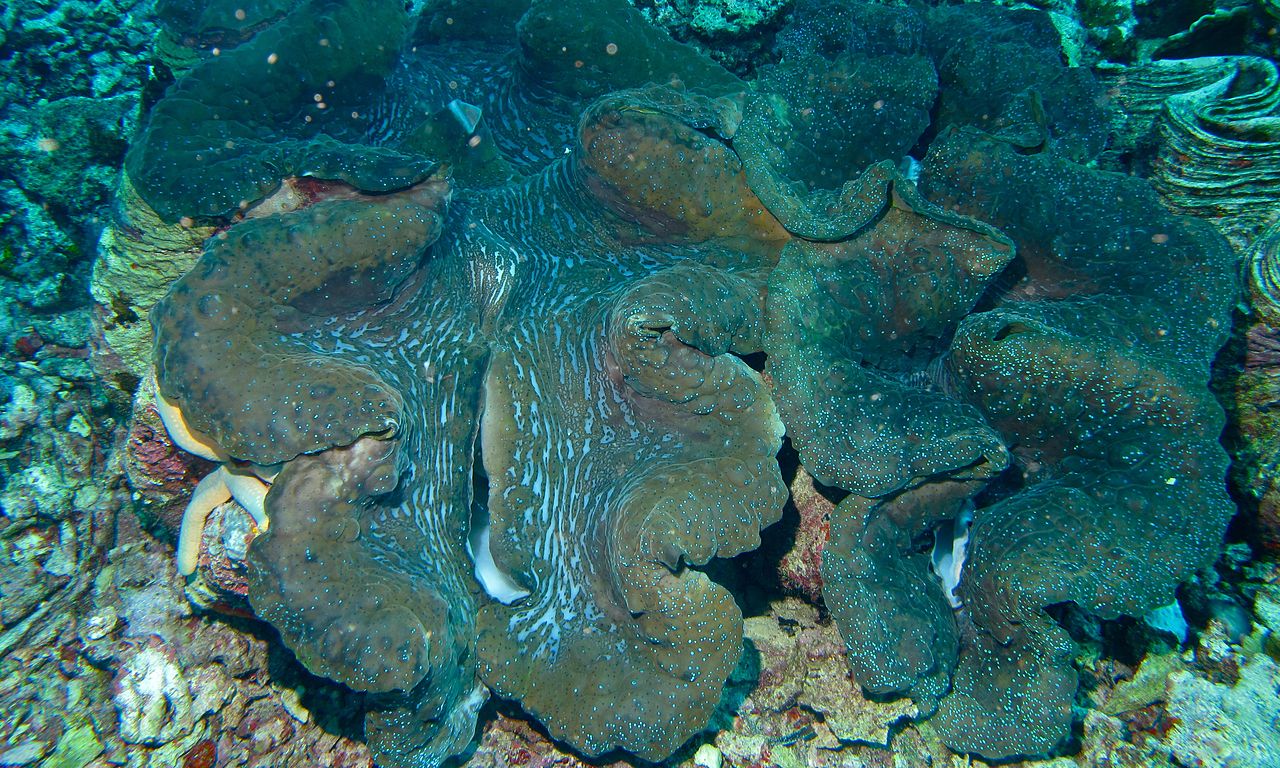
Two Tridacna gigas side-by-side. This species can grow to be almost four feet wide, weigh over four hundred pounds, and live for over one hundred years. Photo by Bernard Dupont; Creative Commons Attribution-Share Alike 2.0 Generic license.
_(6058446919).jpg)
Strontium is also useful for analysis of marine invertebrates. In this case, the utility is closely related to its size at the atomic level: it is almost exactly the same size as a calcium (Ca) atom. Additionally, both elements are alkaline Earth metals, which means they share many of the same properties, like tending to form ions with 2+ charges. In clams like Tridacna (see image above), the Sr:Ca ratio has been demonstrated to reliably capture daily cycles, providing highly detailed information on growth rate during the clams’ lives and their lifespans. In this case, the daily cycles in Sr:Ca are connected to the photosynthetic symbionts living in association with the giant clams because they photosynthesize and respire predictably based on exposure to sunlight and draw in different amounts of strontium and calcium during those processes. Thus, analysis of Sr:Ca ratios can be used to study the timing and dynamics of the coevolution between Tridacna and its algal symbiont.
Though there are still a great many other isotopes that can be applied in paleoecology, and others still that are being developed for new applications, those discussed here are representative of those commonly used. As we expand our knowledge of how organisms use different isotopes and how those isotopes are preserved in the fossil record, we will continue to learn new things about how organisms behaved and interacted in the past. The application of biogeochemical studies and techniques to paleoecology will continue to grow and produce exciting new information for many years to come.
An isotopic example from the clams in the Colorado River estuary
To take a closer look at how isotopic information is developed and applied, this section will discuss an example from the Colorado River estuary. Over the last century, the Colorado River has been dammed extensively in the United States (e.g., Hoover Dam, Glen Canyon Dam) and water has been diverted to major cities (e.g., Las Vegas, Phoenix), to the point where practically no freshwater reaches the downstream estuary. Situated at the north end of the Gulf of California in Mexico, the Colorado River estuary has, undeniably, undergone substantial ecological change as a result of these dams and water diversions. Although it is certain that change has occurred, the scope and magnitude of the change remains unknown because there were no major ecological studies in the estuary prior to the beginning of twentieth century when upstream dam construction began. There are, however, well-preserved deposits of molluscan remains in the estuary, enabling a retrospective assessment of the pre-dam community. Through comparison of the past and presently-living communities, we can begin to understand the extent to which the estuary has changed (learn more about this type of study in the chapter on Conservation Paleobiology). A handful of isotopic studies on clams in the estuary, conducted by David Dettman, Karl Flessa, David Goodwin, Peter Roopnarine, and Bernd Schöne, have helped quantify some of these changes.
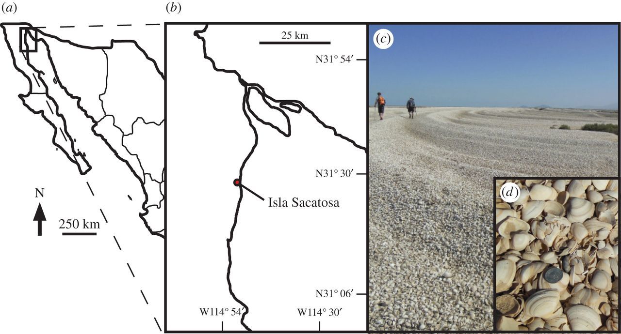
The Colorado River estuary in the northern Gulf of California (Mexico) and the large accumulation of molluscan remains. As estimated by Kowalewski et al. (2000), these accumulations contain more than two trilllions shells! "Cheniers in the Colorado River delta. (a) Location of delta in Mexico. (b) Colorado River delta locality from Kowalewski et al. (2000). (c) A chenier in the Colorado River delta at a locality south of Isla Sacatosa. (d) Close-up of Mulinia coloradoensis; coin, 0.24 cm in diameter." Image and caption from Smith et al. (2016) in Royal Society Open Science; Creative Commons Attribution 4.0 International license.
As is often the case with isotopic studies, these researchers started by examining living individuals to first understand how they live and grow in their current environment. Using oxygen isotopes, they sampled several individuals of the hard clam, Chionista fluctifraga, that had been living in the estuary. Sampling the clams requires cutting one of the valves down the middle, across the growth lines on the shell. Once it is cleaned, the cut interior of the shell reveals tiny growth lines, which can represent growth increments down to the daily scale. Using a small drill—this can also be done using a newer technique called laser ablation—tiny samples of the shell are removed along the shell’s interior and this is where the isotopic data come from. After some preparatory work in the laboratory to clean the samples and isolate the content of interest, the samples of powdered shell are then analyzed using a mass spectrometer, which is the instrument that detects different types of elements and isotopes, and their abundances. Each sample is analyzed and, because the location of each sample on the shell is known, a δ18O profile can be generated.
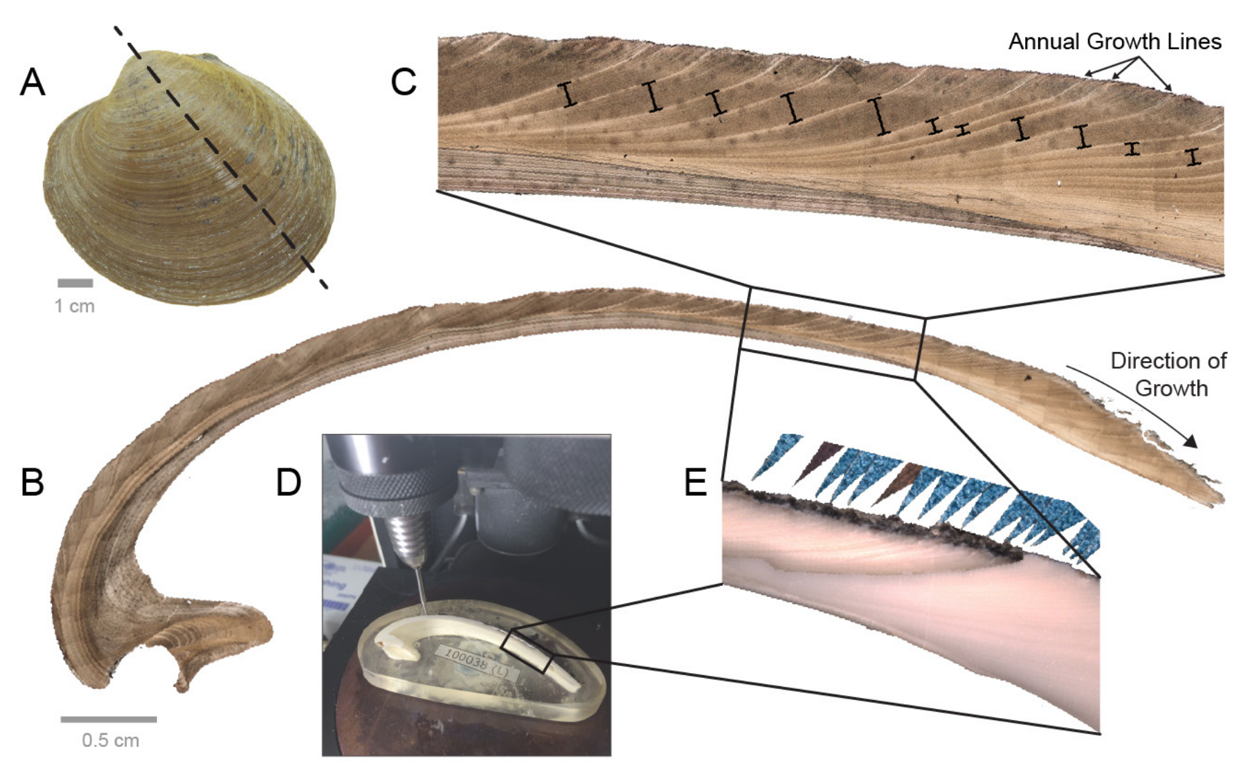
From A to E, a visualization of the process for sampling a clam shell isotopically. "(A) The left valve of an Arctica islandica shell. Dashed line shows maximum growth axis. (B) Photomicrograph of the acetate peel of an A. islandica shell sectioned along the maximum growth axis. (C) Photomicrograph of boxed area in (B), showing annual growth lines and increments (depicted by black bars). (D) Photograph of an A. islandica shell, embedded in an epoxy block and positioned under a micromill. (E) Photograph, in reflected light, of an A. islandica shell, partially milled for oxygen isotopes. This photograph depicts the boxed region in (B) and (D). Annual growth lines are marked by blue triangles." Figure and caption from Wanamaker et al. (2016) in the Variations newsletter of US CLIVAR.
Using this process, the researchers first created growth profiles for two individuals from the estuary. Importantly, because they started with living organisms, they were then able to compare the isotopic profiles derived from the shells with instrumentally measured temperature data for the entire time the clams were alive. This comparison allowed them to closely correlate the clams’ isotopic profiles to the temperature variations. They found that the clams typically started to grow in late March or early April and continued until late November or early December, depending on the year. Additionally, they were able to determine, through comparison to the temperature data, that the clams stopped growing when temperatures decreased below 17° C (~63° F) or increased above 31° C (~88° F).
In the following years, the researchers conducted several more analyses, refining the growth profiles to establish typical growth rates throughout the year and developing a model to describe that growth based on temperature. Only after this careful study and quantification of the living hard clams did the researchers apply their findings to clams from the past. As discussed in the section on oxygen isotopes, temperature can heavily influence the δ18O, as shown in the image above, but salinity also has an impact. Recall that freshwater tends to hold a lower δ18O value than seawater, when holding temperature constant. In the case of the clams in the Colorado River estuary, the researchers first established the effect of temperature on annual growth and then began to explore the influence of salinity.
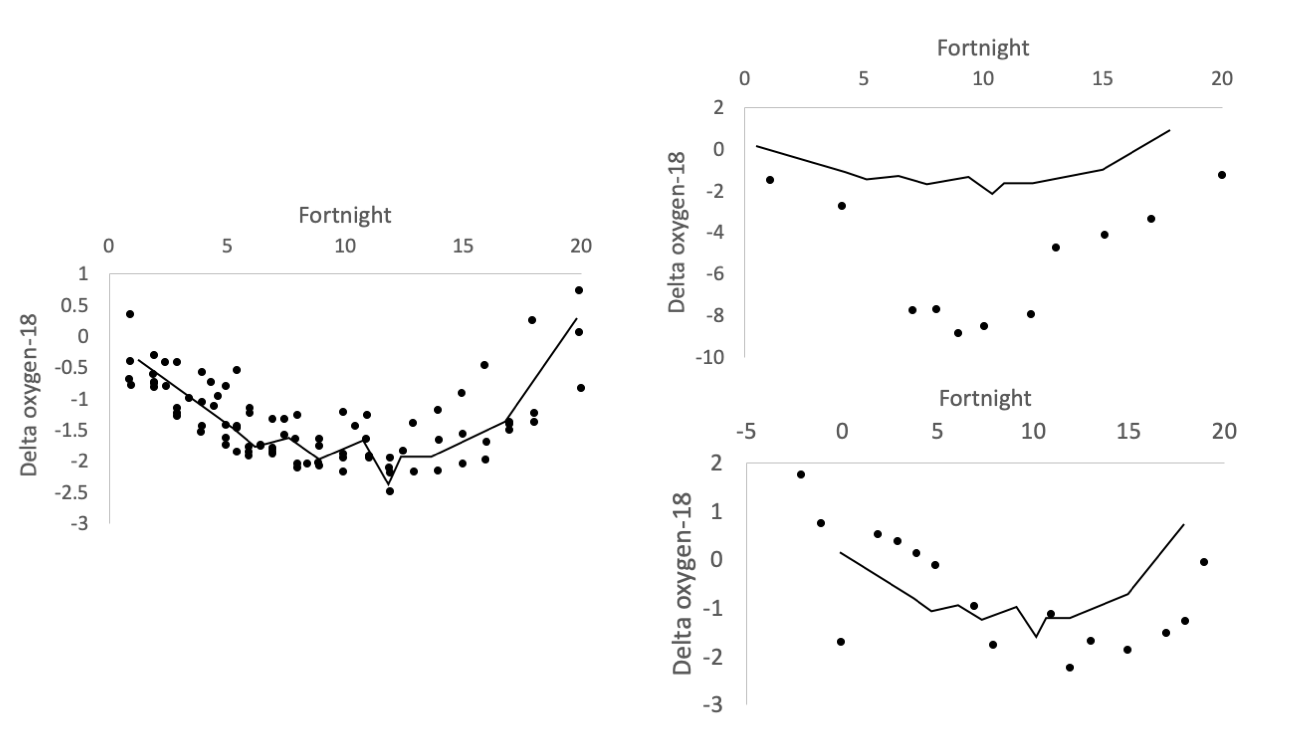
The left image shows δ18O records for live-collected shells in years during which no Colorado River flow occurred. The “no-flow record” (fitted line, which is the same line in each figure) is the average of these by fortnight. The top right image shows the δ18O profile of a shell from 1775 AD, dated using amino acid racemization by Kowalewski et al. (1998), during its third year. There is a strong river water spike in fortnights 7 to 12 and the values are more negative overall, both of which indicate freshwater input. The bottom right image shows the δ18O profile for a shell collected in 1998. There is a small offset, showing a water release from February of that year. Figure redrawn from Dettman et al. (2004) in Geochimica et Cosmochimica Acta.
Although water from the Colorado River has not reached the estuary in recent years, there have been times when freshwater flows were intentionally released. During these times (e.g., 1993, 1998), the researchers were able to sample clams to attain their isotope profiles across these flow releases. The flows were not released with the clams in mind but, in many ways, the freshwater releases can be viewed as experiments from the perspective of clam oxygen isotope profiles. That is, because the amount of water being released was known during these periods of release, the researchers could quantify the impacts of known amounts of freshwater on the clam profiles. For example, from mid-March to mid-December in 1993, 3.10 x 10⁹ m3 of water were intentioanlly released and, using the methods described above, the researchers estimated a similar flow of 2.51 x 10⁹ m3 of water from clam shell isotopes during the same time period. With all these data from recent times, the researchers could then turn to older clams from times in the past when the Colorado River was flowing unimpeded. Using the same oxygen isotopes, and the calibration to the more recent freshwater releases, they could then estimate the amount of water (1.02 x 10¹⁰ m3 of water in one year) that would have been flowing while the clams from the past were living. This body of work, which occurred over several years, provides a novel way to estimate river flow from times in the past prior to instrumental records and, often, prior to human impacts. In the Colorado River estuary, these isotopic records have helped form the basis for more studies of ecological change in the estuary.
An isotopic example from Proboscideans
Proboscideans, which include living elephants and their extinct relatives, are excellent candidates for isotopic analysis because of their robust teeth and the large tusks grown by many members of this group. The teeth and tusks, which are technically the animals’ incisor teeth, grow continuously and record information on where and how the animal was living. Examination of these teeth, with comparison and verification from similar studies of living proboscideans (i.e., elephants), can provide information on what the ancient animals were eating, where they lived throughout the year, and the development of individuals from their early years into adulthood.
If you want to learn more about the evolution of elephants and their relatives, check out the video below!
"The Evolution of Elephants, Mammoths and Mastodons - Proboscidean Family Tree" by Kobean History. Source: YouTube.
Gomphotherium diet and seasonality
In a study on the species Gomphotherium productum, David Fox and Daniel Fisher collected isotopic samples from the tusks of seventeen individuals that lived on the Great Plains of North America during the Miocene epoch to reconstruct their diets. From each tusk, the researchers removed multiple small samples, corresponding to approximately one year of the animals’ lives, and examined their carbon and oxygen isotope profiles. Looking at the δ13C values for these samples, Fox and Fisher found that these large herbivorous animals ate a diet of primarily C3 plants from an arid woodland, as depicted in the image below.
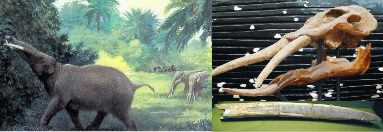
A reconstruction of Gomphotherium in an open woodland habitat (left) with close ups of a Gomphotherium skull (top right) and tusk (bottom left). Left image by Charles Knight (public domain). Top right image by Ghedoghedo; Creative Commons Attribution-Share Alike 3.0 Unported license. Bottom right image by James St. John; Creative Commons Attribution 2.0 Generic license.
_2_(15440055836).jpg)
Interestingly, there was very little variation in the isotope values during the years that were sampled, suggesting a relatively stable source of food for the Miocene Gomphotherium and little environmental variability. To assess seasonality and environmental variability, the researchers also analyzed the δ18O isotope profiles along the tusks and found low-magnitude cyclicity on an annual basis, corresponding to seasonal differences in precipitation. Taken together, the isotopic information suggests small seasonal changes producing wetter and drier periods during the year, but ultimately not enough variation to change the diet of the Gomphotherium.
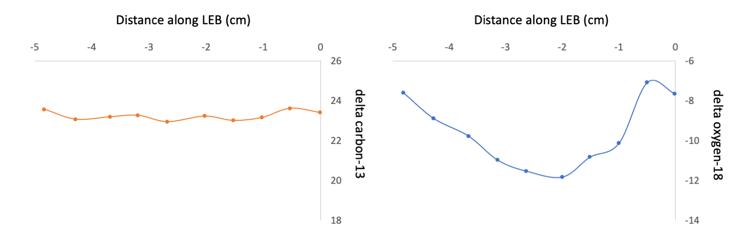
Representative data from the tusk of a Miocene Gomphotherium showing little annual change in δ13C values (left figure), indicating a stable diet, and seasonal variability in δ18O (right figure), suggesting annual variation in precipitation. "Variation in δ13C [left] and δ18O [right] for F:AM 25711 (Rock Ledge Mastodon Quarry, Ash Hollow Formation, Ogallala Group, NE, Late Clarendonian)." Figure redrawn from Fox and Fisher (2004) in Palaeogeography, Palaeoclimatology, Palaeoecology.
Mammoth and mastodon migration
Examining teeth of mammoths and mastodons from the southeastern United States, a team led by Kathryn Hoppe reconstructed potential migrations for these late Pleistocene proboscideans. As discussed earlier in this chapter, strontium isotopes can be used to retrospectively track animal movement because the ratio of 87Sr/86Sr in the environment is recorded proportionately in the teeth and bones of animals. Based on these records in the mammoth and mastodon teeth, plus data on the ratio of 87Sr:86Sr in the bedrock of the southeastern United States, Hoppe and her team reconstructed the movements of these animals.
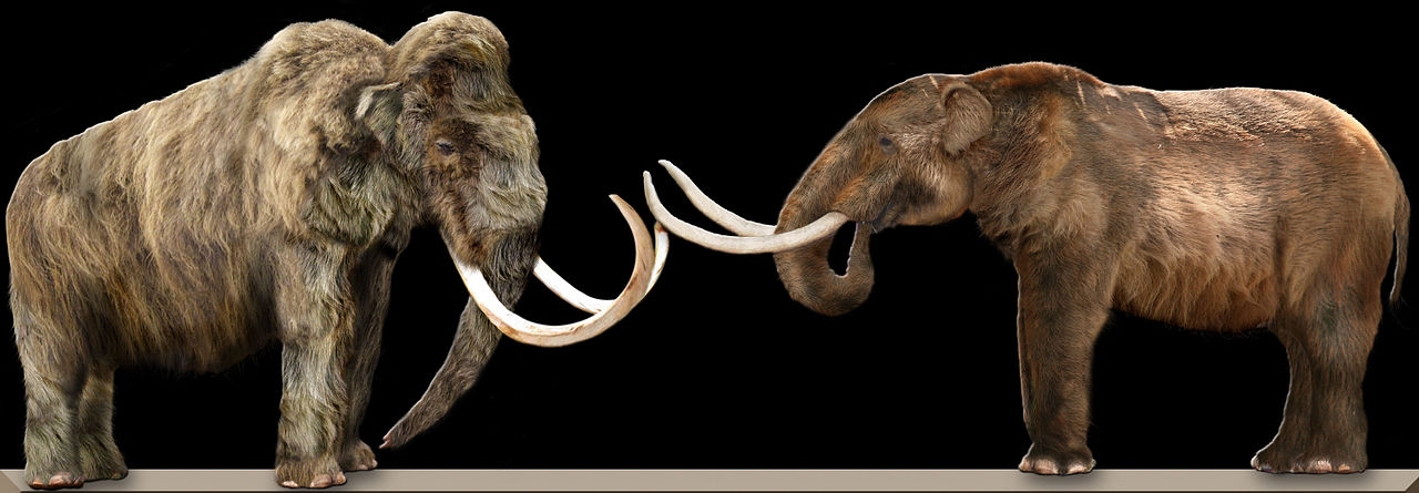
A side-by-side comparison of a mammoth (left) and mastodon (right), two extinct proboscidean relatives of living elephants. Image by Dantheman9758; Creative Commons Attribution-Share Alike 3.0 Unported license.
Bedrock strontium ratios in southern and coastal Florida—and extending northward up the Atlantic coast—are relatively low due to their carbonate composition. In comparison, the more northern and continental bedrock in the southern Appalachians of Georgia is composed of metamorphic and igneous rocks, carrying a higher 87Sr/86Sr ratio. When analyzing the strontium ratio in the mammoth and mastodon teeth, two different patterns emerged. For mammoths, there was very little change in the ratio; however, for mastodons, the majority of individuals showed variation between higher and lower ratios. These results suggest that mastodons very likely migrated between southern, coastal Florida and the inland region in Georgia. These movements may represent an annual migration pattern, but this conclusion cannot be reached with absolute certainty due to time-averaging of the assemblage. Comparisons with living elephants suggest that the movements may have occurred on an as-needed basis. The feeding behaviors of elephants can be highly destructive and, because they require a large number of calories, elephants can quickly strip an area of vegetation. Hoppe and her team suggest that this may have been true of mastodons as well.
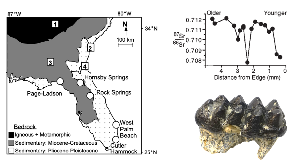
The left image shows the regions with different strontium ratios: the black and gray zones have similarly high values with the white zone being lower. The top right image shows the strontium profile of a mastodon tooth (depicted in bottom right), with the variation indicating that the individual moved between regions of different bedrock strontium ratios during its life. Left image caption: "Bedrock geology of Florida and Georgia showing locations of modern rodent sites (squares) and fossil quarries (circles). Average 87Sr/86Sr ratios of modern rodents sites are (1) 0.7143 ± 0.0004, (2) 0.7092 ± 0.0000, (3) 0.7117 ± 0.0016, (4) 0.7087 ± 0.0015. Average 87Sr/86Sr ratios of modern plants collected at fossil sites are Page-Ladson, 0.7090 ± 0.0001; Hornsby Springs, 0.7095 ± 0.0003; and Rock Springs, 0.7085 ± 0.0004. Top right image caption: "87Sr/86Sr ratios of microsamples from Page-Ladson mastodon #148668. Samples are inferred to represent approximately two years of growth based on variations in thickness of growth line." Left and top right images from Hoppe et al. (1999) in Geology (Special "Fair Use" permission). Bottom right image by Daderot; Creative Commons CC0 1.0 Universal Public Domain Dedication.
The mammoth tooth strontium ratios are somewhat harder to interpret. Whereas mastodons were browsers and ate from trees and shrubs, mammoths were primarily grazers and ate grasses. Though their strontium profiles do not show significant change, it is possible that the mammoths were able to track their preferred habitat and food along the Atlantic coast of the United States. That is, mammoths might have migrated just as far as their mastodon counterparts, but it might not be recorded by the strontium isotope ratio because the ratio remained constant in the area over which they migrated. Based on the strontium isotopes, it is likely that mastodons migrated several hundred kilometers on a regular basis and, although it is possible that mammoths also migrated, it is more parsimonious to conclude that they were not as nomadic as contemporary proboscideans or their living relatives.
Mammoth life history
The continuous growth of tusks allows paleontologists to assess patterns in the growth and development of individuals. In addition to information on growth rate and life span, tusks record the juvenile years of mammoths—and other proboscideans—and can be examined to determine how long young mammoths fed on milk from their mothers. Consumption of milk can be detected using a variety of isotopes, but nitrogen provides one of the clearest signals because δ15N increases at each trophic level. Though it may seem counterintuitive to consider a milk-fed juvenile at a higher trophic level than its mother, this is a consequence of the way animals process and accumulate the heavier nitrogen isotope—and a convenient one for paleontologists.
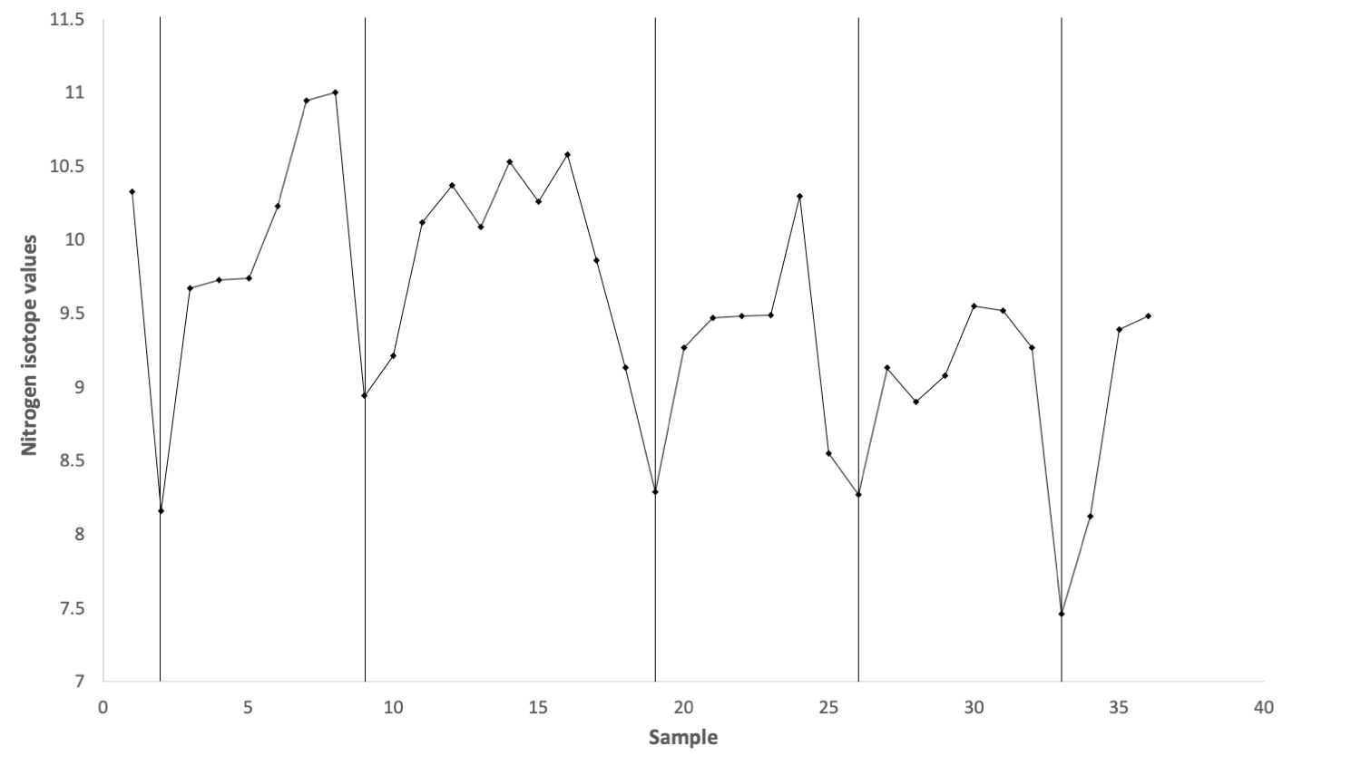
Profile of δ15N from the juvenile mammoth tusk found on Wrangel Island. The vertical black lines indicate years; this individual was at least five years old. Increasing sample number (on the x-axis) is representative of length from the tip to the base of the tusk. This figure was created from the data published in Table 1 of Rountrey et al. (2007) in Quaternary International.
Taking advantage of this relationship, Adam Rountrey and his collaborators sampled the tusk of a juvenile woolly mammoth from Wrangel Island, off the northern coast of Russia, that likely lived between three and nine thousand years ago. This remote island served as a refuge for mammoths, as this population likely was the last to die out and outlasted mainland populations by several thousand years. The δ15N values from the tusk show an annual cycle, indicating the juvenile was likely six years old when it died. Notably, the cycle shows a decreasing δ15N value year after year, which is consistent with a weaning period where the juvenile relies less and less on its mother’s milk. Today, most elephants wean their young over a period of three to four years, but the timing can approach six years in harsh climatic conditions. Given the northern, arctic climate on Wrangel Island, it is likely that the juvenile was reliant on its mother’s milk for an extended period because of the harsh climate there. This extended weaning period has important implications for the mammoth population because, when a mother is nursing, she will not produce another offspring. Consequently, the growth rate of the population will slow down. It is not clear whether this decrease in population growth rate contributed to the extinction of this species, but it is plausible that it would have made the population more susceptible to changing climate and predation by humans.
Concept check: See what you know!
What is an isotope?
An isotope is an atom containing a greater or lesser number of neutrons than typically found in an atom of the element (e.g., carbon-13; oxygen-18)
Name three ways paleoecologists use isotopes to understand the past.
Isotopes can be used to study past temperatures, rainfall amounts, and salinity. Additionally, isotopes can tell us about trophic structure, behaviors such as being nocturnal or semi-aquatic, evolution of life, growth rates, and more.
True or false: Animal hard parts (e.g., teeth, bones, shell) tend to incorporate Oxygen isotopes in the proportion that the isotopes occur in the animal's environment.
True
Which isotope would you study if you wanted to know an animal's trophic level: oxygen, carbon, or nitrogen?
To understand trophic level, nitrogen isotopes would be the best choice. At each increasing trophic level, the ratio of nitrogen-15 to nitrogen-14 increases by 2-4%.
Which isotope would you study if you wanted to you when life first evolved on earth: oxygen, carbon, or nitrogen?
To understand when life first evolved, carbon isotopes would be the best choice. Life forms tend preferentially use carbon-12 over carbon-13 because it is lighter and easier to use. Consequently, the ratio of these isotopes in organisms is often different from their inorganic surroundings.
References and Further Reading
Barrick, R. E. 1998. Isotope paleobiology of the vertebrates: ecology, physiology, and diagenesis. The Paleontological Society Papers, 4: 101-137.
Bell, E. A., P. Boehnke, T. M. Harrison, and W. L. Mao. 2015. Potentially biogenic carbon preserved in a 4.1 billion-year-old zircon. Proceedings of the National Academy of Sciences, 112: 14518-14521.
Clementz, M. T. 2012. New insight from old bones: stable isotope analysis of fossil mammals. Journal of Mammalogy, 93: 368–380.
Dettman, D. L., K. W. Flessa, P. D. Roopnarine, B. R. Schöne, and D. H. Goodwin. 2004. The use of oxygen isotope variation in shells of estuarine mollusks as a quantitative record of seasonal and annual Colorado River discharge. Geochimica et Cosmochimica Acta, 68: 1253-1263.
Elliot, M., K. Welsh, C. Chilcott, M. McCulloch, J. Chappell, and B. Ayling. 2009. Profiles of trace elements and stable isotopes derived from giant long-lived Tridacna gigas bivalves: potential applications in paleoclimate studies. Palaeogeography, palaeoclimatology, palaeoecology, 280: 132-142.
Fox, D. L., and D. C. Fisher. 2004. Dietary reconstruction of Miocene Gomphotherium (Mammalia, Proboscidea) from the Great Plains region, USA, based on the carbon isotope composition of tusk and molar enamel. Palaeogeography, Palaeoclimatology, Palaeoecology, 206: 311–335.
Goodwin, D. H., B. R. Schone, and D. L. Dettman. 2003. Resolution and fidelity of oxygen isotopes as paleotemperature proxies in bivalve mollusk shells: models and observations. Palaios, 18: 110-125.
Hoppe, K. A., P. L. Koch, R. W. Carlson, and S. D. Webb. 1999. Tracking mammoths and mastodons: reconstruction of migratory behavior using strontium isotope ratios. Geology, 27: 439-442.
Norris, R. D., and R. M. Corfield. (eds.). 1998. Isotope paleobiology and paleoecology. Paleontological Society, New Haven. 285 pp.
Rountrey, A. N., D. C. Fisher, S. Vartanyan, and D. L. Fox. 2007. Carbon and nitrogen isotope analyses of a juvenile woolly mammoth tusk: evidence of weaning. Quaternary International, 169: 166-173.
Schöne, B. R., J. Lega, K. W. Flessa, D. H. Goodwin, and D. L. Dettman. 2002. Reconstructing daily temperatures from growth rates of the intertidal bivalve mollusk Chione cortezi (northern Gulf of California, Mexico). Palaeogeography, Palaeoclimatology, Palaeoecology, 184: 131-146.
Trench, R. K., D. S. Wethey, and J. W. Porter. 1981. Observations on the symbiosis with zooxanthellae among the Tridacnidae (Mollusca, Bivalvia). The Biological Bulletin, 161: 180-198.
Yamanashi, J., H. Takayanagi, A. Isaji, R. Asami, R., and Y. Iryu. 2016. Carbon and oxygen isotope records from Tridacna derasa shells: toward establishing a reliable proxy for sea surface environments. PloS ONE, 11: 1-19.
Usage
Unless otherwise indicated, the written and visual content on this page is licensed under a Creative Commons Attribution-NonCommercial-ShareAlike 4.0 International License. This page was written by Jansen A. Smith. See captions of individual images for attributions. See original source material for licenses associated with video and/or 3D model content.
