
Chapter contents:
Conservation Paleobiology
– 1. Foundations in Conservation Biology
– 2. Approaches in Conservation Paleobiology
–– 2.1 Near-time Approaches
–– 2.2 Deep-time Approaches ←
– 3. Deliverables from Conservation Paleobiology
– 4. Barriers to Applying Conservation Paleobiology
Above image by Photolitherland; Creative Commons Attribution 3.0 Unported license.
Introduction
Deep-time approaches in conservation paleobiology are less systematically pursued than near-time approaches. Though the deep-time record—which includes everything older than 2.6 million years—can contribute to conservation practice, it is not used in the same way as the near-time record. For instance, many of the species found in the deep-time record have gone extinct, making it challenging to draw direct comparisons with species, communities, and ecosystems of today. The absence of one species, Homo sapiens, in the deeper record represents another particularly substantive difference. Today, people are the main drivers of environmental change and so inferences from a pre-human time must be considered carefully before potentially being applied in conservation. Likewise, the possibility of extensive time-averaging and taphonomic bias require extra attention with deep-time approaches. Whereas the near-time record tends to be averaged over hundreds or thousands of years, the deep-time record can be averaged over tens of thousands, hundreds of thousands, or millions of years. Additionally, taphonomic processes have been acting on the deep-time record for longer, increasing the possibility for alteration. Daunting though it may seem, these variables can be assessed, and the deep-time record can be used to understand and improve conservation practice.
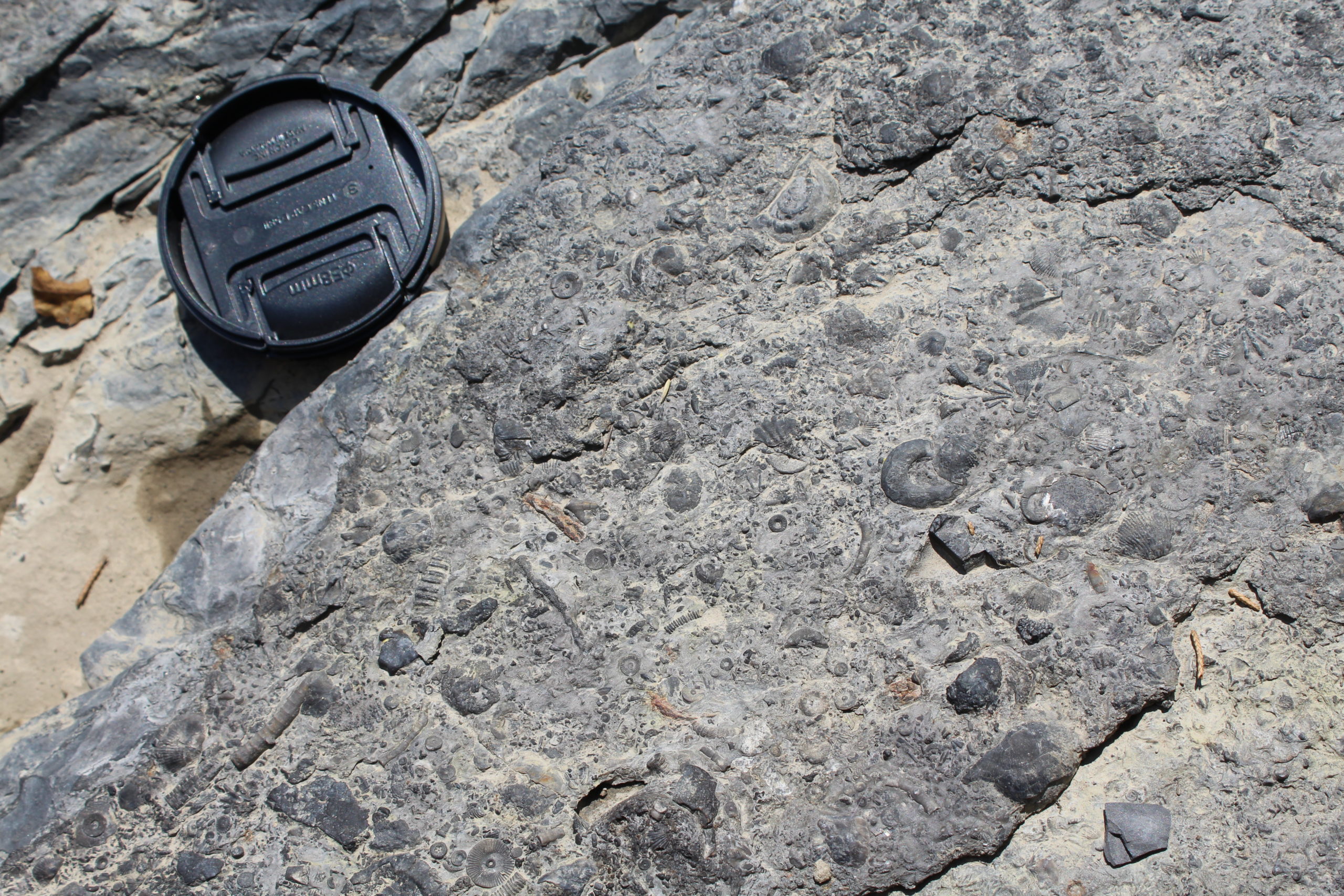
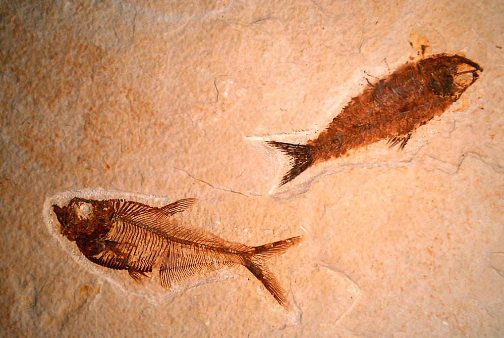
Devonian fossils from upstate New York. Fossils like these have been studied to understand stability in community structure in response to changing habitats through time. Photo by Jansen Smith.
One of the greatest strengths of this approach is the multitude of “experiments” held in the record from the last several hundreds of millions of years. Though they were not driven by humans, many of the same environmental stressors afflicting ecosystems today (e.g., climate change, eutrophication, habitat change) also influenced life in the past. Whereas the future consequences of these stressors are uncertain in current times, the long-term effects have already played out in the deep-time fossil record. The species may have been different but factors like the timeframe of recovery and general patterns of extinction in the past can be used to build scenarios for what we might expect to see in the coming decades and centuries. In this way, the deep-time fossil record can help us prepare for a set of potential futures and help guide our decision making towards preferable scenarios. In the examples that follow, we will explore a few ways the deep-time record has already helped us understand what the future may hold.
Understanding extinctions
The sixth mass extinction
We are in the early stages of a mass extinction, but what does that mean?
Extinction—the death of all individuals in a taxonomic group (e.g., species, genus)—is a natural process that occurred repeatedly in the history of life, and still occurs in the world around us today. A great many factors can contribute to the extinction of a species (e.g., climate change, competition, eutrophication, ocean acidification, predation, etc.) and, generally, the factors all amount to a relative loss of fitness—the capacity to survive and reproduce (learn more in the chapter on Evolution). In a technical sense, extinction occurs when the last individual of a species dies; however, this final death is often preceded by centuries, millennia, or millions of years of decline in population size, population density, and/or geographic range. The constant extinction of species through time is often referred to as “background” extinction, acknowledging that evolutionary processes are constantly at work. For most of the history of life on Earth, this background extinction is matched, if not exceeded, by the origination of new species (learn more about Speciation). Mass extinctions can be thought of as an imbalance between extinction and origination.
"What Does The Sixth Mass Extinction Mean for Humans" by Second Thought. Source: YouTube.
In the past history of life, five mass extinctions have been recognized—and arguably another occurred at the end of the Ediacaran (542 mya) but this is not yet commonly counted. These events changed the trajectory of life on Earth when they occurred at the ends of the Ordovician (450 – 440 mya), Devonian (375 – 360 mya), Permian (~252 mya), Triassic (~201 mya), and Cretaceous Periods (~66 ma). During each of these times, at least 75% of species on Earth went extinct over relatively short periods of time; the rates of extinction during these times were much greater than the concurrent rates of species origination. By comparing the rates of extinction during these times with the rate at which species are currently going extinct, the deep-time fossil record can contextualize the biodiversity crisis we find ourselves in today.
"Mass Extinctions" by SciShow. Source: YouTube.
In 2011, a team of researchers led by Anthony Barnosky published a paper detailing just such a comparison. They found, in all of their numerous comparisons, that we are undeniably on pace for another mass extinction unless substantial action is taken to alleviate the loss of species. Because the comparisons were between events occurring over durations of millions of years in the past and only centuries or millennia in the present, they standardized their rates to “extinctions per million-species-year” (E/MSY). Illustratively, an E/MSY of one would mean that if there were one million species alive today, one would go extinct each year. If we consider the last 1,000 years, the E/MSY has been 24. The average from the fossil record is 1.8 E/MSY. This comparison suggests that we are very likely experiencing the early stages of a mass extinction. Barnosky et al. (2011) also estimated the amount of time needed to reach mass extinction level die offs (i.e., > 75% of species) based on their estimated rates of contemporary extinction. With no modifications to current human behavior, we will reach that threshold in 240–540 years. With more optimistic assumptions, the threshold is pushed to 11,330 years from now. Regardless, the future of many species on Earth is bleak without substantial changes to the human status quo.
Troubling as their findings are, Barnosky et al. (2011) do add, optimistically, that we have not yet technically experienced the mass extinction. Though the rate of extinction is consistent with a mass extinction, we are a long way off from losing 75% of species. If we are to avoid another mass extinction, the fossil record tells us that we must act swiftly.
Identifying at-risk species
The fossil record can help us to identify modern species with elevated risk of extinction and this information can be used to prioritize conservation effects. Working towards this goal, a team of researchers led by Seth Finnegan examined data on the extinction of 2,897 marine genera from six taxonomic groups—bivalves, gastropods, echinoids, sharks, mammals, and scleractinian corals—over the last 23 million years. Finnegan et al. (2015) found that geographic range size and taxonomic identity were consistently the best predictors for the extinction of fossil genera. Genera with smaller geographic ranges were more susceptible to extinction than those with broader ranges, as they are also likely more sensitive to habitat loss, local disturbance, and environmental change. Taxonomic identity reflects the shared evolutionary history of the different groups and their associated common traits and life histories, making it unsurprising that this variable was an important predictor. Certain groups of corals (e.g., faviids), which tend to have high rates of endemism and restricted geographic ranges, were highly susceptible, as were some mammals (e.g., cetaceans).
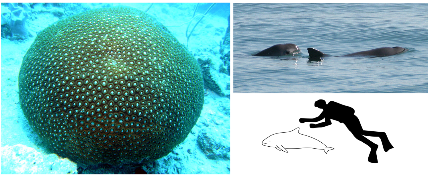
A Favia coral (left), belonging to the Faviidae family and a rare image of the vaquita porpoise (top right). The tiny vaquita (compared to a human, lower right) is endemic to the northern Gulf of California and its population is below 15 individuals. Left image by Anders Poulsen, Deep Blue; Creative Commons Attribution-Share Alike 3.0 Unported license. Top right image by Paula Olson, NOAA (public domain). Bottom right image by Chris_huh; GNU Free Documentation License.
Another important factor in the analysis by Finnegan et al. (2015) was the region were genera lived. Most commonly, the genera with the highest susceptibilities were found in tropical regions for most taxonomic groups—gastropods from Antarctica appear to be most susceptible, likely due to their endemism. When the researchers also considered the distributions of human impacts and effects of climate change, this pattern appears to be even more problematic. The tropics experience more human impacts and greater effects of climate change. Coupled with the finding that genera are already highly susceptibile in this region, the prognosis for modern tropical marine genera is not an optimistic one. Based on the work of Finnegan et al. (2015), conservationists should prioritize tropical marine genera, particularly corals and mammals.
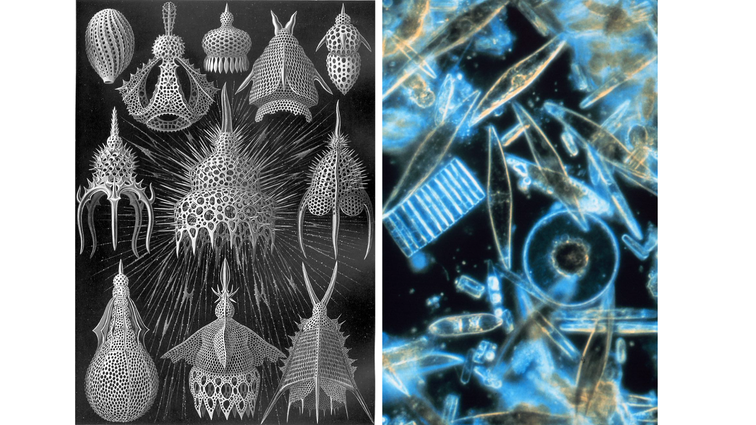
An assortment of radiolarians (left) and diatoms (right) such as those used in the study by Smit and Finnegan (2019). Left image by Ernst Haeckel (public domain). Right image by Prof. Gordon T. Taylor, Stony Brook University (public domain).
Models of extinction in the past are based on organisms that are no longer living today whose remains are subject to taphonomic bias and time-averaging. These differences raise the question, how reliable are models based on long-dead organisms for predicting modern extinction?
To address this question, Smit and Finnegan (2019) examined the extinction of calcareous nannoplankton, diatoms, planktonic foraminifera, and radiolarians during the last 63 million years. Using these groups, Smit and Finnegan built four different models to explain species extinctions. The models were then parameterized using information from preceding periods of the past to predict extinct risk in the subsequent record. That is, even though all of their data were from the past, they used portions of those data to predict the extinction likelihood for species occurring more recent in the geological record, analogously to us now using the fossil record to understand species extinctions today. Depending on which of the four models was assessed, this approach was able to correctly predict extinction risk between 70% and 80% of the time. Though limited in the scope of the taxa considered, this work is a positive indicator that the fossil record can be used to reliably model future extinction risk. By taking advantage of the deep-time record in this way, conservationists can improve their ability to evaluate extinction risk today.
Trends across the Paleocene-Eocene Thermal Maximum
The Paleocene-Eocene Thermal Maximum (PETM), which occurred approximately 56 million years ago, was a period of rapid climate warming similar to that which we are experiencing today. During the PETM, massive amounts of carbon were released into the oceans and atmosphere over a relatively short period of time (<10,000 years). The release of this carbon resulted in a rapid temperature increase, of 5 – 9 °C (or 8 – 15 °F), due to the same greenhouse effects we experience today. Because of its similarity, biological responses to the warming climate during the PETM are often used to set expectations for how plants and animals will respond to current climate change. In the following examples, we will consider the body size of horses and insect-plant interactions while exploring how the deep-time record can help us understand what may lie ahead in our warmer future.
Tiny horses during the PETM
One of the responses that has been predicted for modern climate change is a decrease in animal body size. This prediction is based on Bergmann’s Rule—named for the nineteen century German biologist, Carl Bergmann, who was one of the first to recognize the pattern—which states that in taxonomic groups (e.g., clades, species, populations), individuals of larger sizes will be found in colder regions whereas smaller individuals will occur in warmer regions. This rule is often considered as a consequence of latitude, with smaller individuals found in the low-latitude tropics and larger individuals in the cooler high-latitude regions.
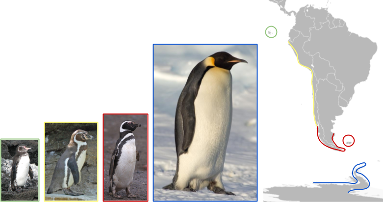
To illustrate Bergman's Rule, we can consider the Galapagos (left-most, green outline), Humboldt (second from left, yellow outline), Magellanic (second from right, red outline), and Emperor (right-most, blue outline) penguins above. Moving from north to south, the penguin species found along South America and in Antarctica (shown in colors matching outlines of the different species) reach larger and larger sizes as the climate grows increasingly colder towards the south. Image by Dorena Nagel.
Bergmann’s rule has been translated to apply to the current climate warming Earth is experiencing. As Earth warms, animals will likely get smaller. Though this prediction is supported by theory, Janet Gardner and her colleagues (2011) found that there is very little evidence to support it. In large part, the lack of evidence is due to the temporal limitation of biological studies. Biological studies typically taken place over a few years, or maybe a few decades, but evolutionary processes tend to play out on longer timescales (e.g., centuries, millennia). Consequently, data with a longer temporal perspective are needed to confirm the prediction that body sizes will decrease. Whereas the near-time record can be used to test this prediction for living species, the deep-time record can be consulted to understand how species from the past responded to similar periods of climate warming.
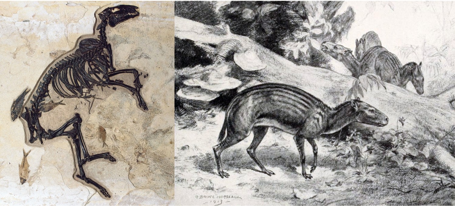
The skeleton of a small, early horse (left) and a reconstruction of early horses browsing in the understory of a forest. Left image from the U.S. National Park Service (public domain). Right image by Bruce Horsefall (public domain).
Horses, which first evolved during the early stages of the PETM, have an excellent fossil record during and after this period of extensive climate warming. Examining the record for the first horse genus, Sifrhippus, Ross Secord and his collaborators (2012) found that these early horses decreased in size by approximately 30%. Though they were small to begin with, likely weighing around twelve pounds, Sifrhippus from the height of the PETM weighed only eight pounds—the size of a small house cat. This decrease in size evolved over 130,000 years and thousands of generations. This long timespan confirms that the size change was an evolutionary response, as it was sustained and directly linked to the warming climate. In contrast, body size changes observed in living organisms have occurred on a decadal scale, in most cases. Because the modern changes have been short-lived (so far), it is difficult to determine whether they are truly evolutionary changes (i.e., shifts in the distribution of alleles in the animal populations) or simply changes within the animals’ existing range of phenotypic variability (i.e., no genetic changes). Based on the evolution of the early horses, it is reasonable to hypothesize that we are observing the beginnings of evolutionary changes in modern animals.
The evolutionary decrease in body size of horses during the PETM supports the assertion of Gardner and her colleagues suggesting that decreased body size is a universal response to climate warming. From a conservation perspective, this is important information because smaller individuals have different energy and water requirements than larger individuals. In particular, smaller individuals are more susceptible to dehydration and heat exhaustion under high temperatures. With this in mind, and with support from data on horse evolution, the deep time record confirms that we should expect these issues to become more prevalent in the coming years. In turn, this information can be incorporated into conservation scenarios of the future to improve our decision-making ability.
Insect herbivory across PETM
As the climate warms, species distributions are shifting as organisms track their preferred environmental conditions. Examples have already been documented for organisms belonging to most branches on the tree of life. Whereas some of these range shifts are likely to be innocuous, and others may even be beneficial, the geographic distributions of many pests and pathogens with negative behaviors and attributes are expanding. These pests and pathogens can reduce standing crop yields by up to 16%, and an equal amount post-harvest, making it important to understand the behavior of these troublesome organisms. Daniel Bebber and his collaborators (2013) examined the spread of these organisms to better understand the threat they may pose to global food security in the not-so-distant future. They noted that, in the Northern Hemisphere, species belonging to Coleoptera (beetles) and Lepidoptera (moths and butterflies) have shifted northward but nematodes (small worm-like organisms) and viruses have shifted southward. On average, Bebber et al. found species were shifting at a rate of 26.6 kilometers each decade. Whereas it is clear that pestilent organisms are spreading, the consequences remain the subject of conjecture.

A caterpillar (left) and beetle (right) eating the margins of leaves. Left photograph by Toby Hudson; Creative Commons Attribution-Share Alike 3.0 Unported license. Right photograph by Cfp: Creative Commons Attribution-Share Alike 2.5 Generic, 2.0 Generic and 1.0 Generic license.
Just as with understanding body size trends in response to climate warming, the deep-time record can help us understand the consequences of pest spread. In the fossil record, traces of insect herbivory on plants are often preserved and can be used to assess specific insect-plant interactions or the frequency of herbivory in general (learn more about Insect Herbivory). Evaluating data compiled from a handful of studies on insect herbivory during the PETM, Ladandeira and Currano (2013) found unequivocal evidence showing an increase in herbivory associated with increasing global temperatures. Independent of the geographic location (e.g., northern Europe, South America, North America), and other factors like ecosystem structure and complexity, both the frequency and diversity of insect-plant herbivory increased. Compared to the time periods before and after the PETM, there were more herbivorous insects eating more plants in more ways. Applying this to today’s climate warming, Ladandeira and Currano (2013) were concise in describing the consequence. They state: “the fossil record makes it clear that elevated insect herbivory in natural and managed ecosystems will be a consequence of current anthropogenic increases in temperature and [carbon dioxide concentrations].”
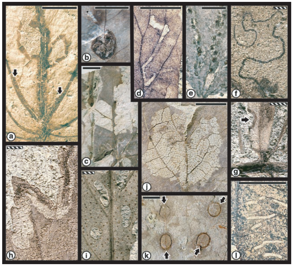
A variety of insect-plant interaction traces from the Williston Basin of southwestern North Dakota. These fossils are from the Cretaceous-Paleogene extinction boundary (~66 million years ago) and are similar to the traces found during the PETM. (a) Two linear mines with oviposition sites (arrows), following secondary and then primary venation, terminating in a large pupation chamber, (b) Single gall on primary vein, (c) Free feeding, (d) Skeletonization, (e) Multiple galls, (f) Initial phase of a serpentine mine, (g) Cuspate margin feeding, (h) Serpentine leaf mine, (i) Hole feeding pattern, (j) General skeletonization, (k) Large scale-insect impressions, (l) Slot hole feeding. Scale bars: solid 1 cm, backslashed 0.1 cm. Figure from Labandeira et al. (2002) in the Proceedings of the National Academy of Sciences under the PNAS License to Publish (Copyright (2002) National Academy of Sciences).
In many places, the effects of increased herbivory have already manifested. For example, in the western United States tree boring beetles have killed thousands and thousands of pine trees. Once killed off by cold winter temperatures, more beetles now survive the warmer winters and their population has expanded rapidly as a consequence. In addition to killing trees, the beetles are indirectly contributing to increasing wildfire intensity, reducing carbon storage in forests, and changing watershed dynamics. These beetles and thier herbivory on pine trees is having devasting effects. The fossil record tells us that this will be the new normal; it is not an exception. Conservation—and agriculture—practices need to carefully address the spread of pests like the pine borer beetle and the possibility that they will have wide-ranging effects on ecosystems, beyond simply decimating plant communities.
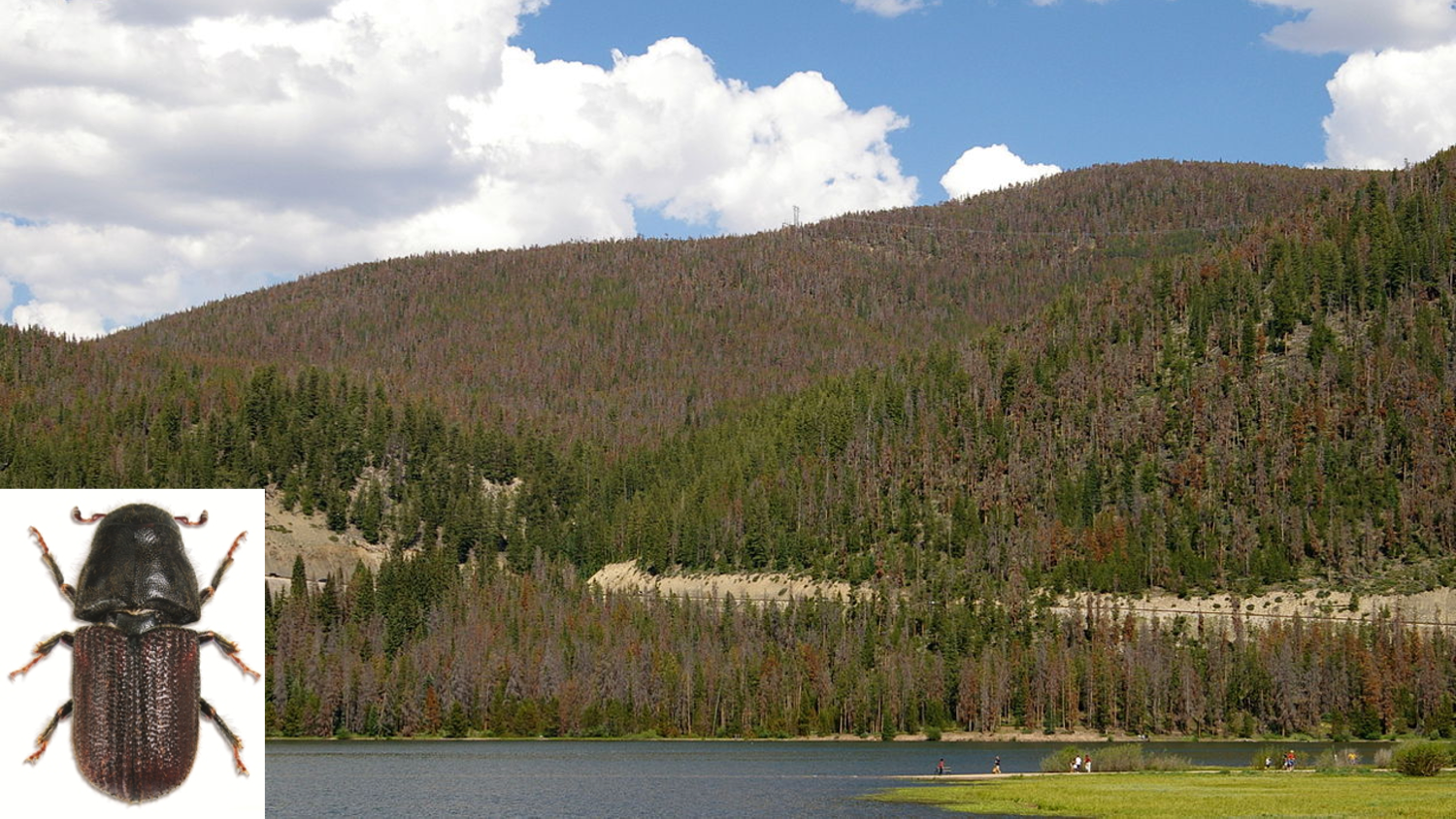
The Rocky Mountain Pine Beetle (lower left) is one of the beetles devastating forests in the western United States. The forest (background) is full of trees that have died as a result of the beetles. Lower left photo by Steve Clarkson (public domain). Background photo by Hustvedt; Creative Commons Attribution-Share Alike 3.0 Unported license.
Concept check: See what you know!
The deep-time record includes everything older than ___ million years.
2.6
What are two ways the deep-time record can contribute to modern conservation practice?
(1) identifying species that are potentially at risk of extinction because they share characteristics with species that have gone extinct in the fossil record; (2) informing scenarios for how species with respond to climate change based on the responses of species in the fossil record to similar circumstances
In order for an extinction event to be classified as a "mass extinction," ___ percent of species have to die out.
According to Bergmann's Rule, where would you expect to find larger species, tropical or polar regions?
Bergmann's Rule says that species (belonging to the same genus or family) found in polar regions will be larger than those in tropical regions.
Applying Bergmann's Rule, how will species sizes change as the climate warms?
Based on Bergmann's Rule, we can predict that species sizes will decrease under warmer climatic conditions.
References and Further Reading
Barnosky, A. D., N. Matzke, S. Tomiya, G. O. Wogan, B. Swartz, T. B. Quental, et al. 2011. Has the Earth’s sixth mass extinction already arrived? Nature, 471: 51-57.
Bebber, D. P., M. A. Ramotowski, and S. J. Gurr. 2013. Crop pests and pathogens move polewards in a warming world. Nature Climate Change, 3: 985.
Dietl, G. P. 2019. Conservation palaeobiology and the shape of things to come. Philosophical Transactions of the Royal Society B, 374: 20190294.
Finnegan, S., S. C. Anderson, P. G. Harnik, C. Simpson, D. P. Tittensor, J. E. Byrnes, et al. 2015. Paleontological baselines for evaluating extinction risk in the modern oceans. Science, 348: 567-570.
Gardner, J. L., A. Peters, M. R. Kearney, L. Joseph, and R. Heinsohn. 2011. Declining body size: A third universal response to warming? Trends in Ecology & Evolution, 26: 285-291.
Keller, G., P. Mateo, J. Punekar, H. Khozyem, B. Gertsch, J. Spangenberg, A. M. Bitchong, and T. Adatte. 2018. Environmental changes during the cretaceous-Paleogene mass extinction and Paleocene-Eocene thermal maximum: Implications for the Anthropocene. Gondwana Research, 56: 69-89.
McInerney, F. A., and S. L. Wing. 2011. The Paleocene-Eocene Thermal Maximum: A perturbation of carbon cycle, climate, and biosphere with implications for the future. Annual Review of Earth and Planetary Sciences, 39: 489-516.
Labandeira, C. C., and E. D. Currano. 2013. The fossil record of plant-insect dynamics. Annual Review of Earth and Planetary Sciences, 41: 287-311.
Secord, R., J. I. Bloch, S. G. Chester, D. M. Boyer, A. R. Wood, A. R., S. L. Wing, M. J. Kraus, F. A. McInernery, and J. Krigbaum. 2012. Evolution of the earliest horses driven by climate change in the Paleocene-Eocene Thermal Maximum. Science, 335: 959-962.
Smits, P., and S. Finnegan. 2019. How predictable is extinction? Forecasting species survival at million-year timescales. Philosophical Transactions of the Royal Society B, 374: 20190392.
Usage
Unless otherwise indicated, the written and visual content on this page is licensed under a Creative Commons Attribution-NonCommercial-Share Alike 4.0 International License. This page was written by Jansen A. Smith. See captions of individual images for attributions. See original source material for licenses associated with video and/or 3D model content.
