

Section contents
Paleoclimate estimation with plant fossils
- Nearest living relative methods
- Leaf margin analysis ←
Related pages & background reading
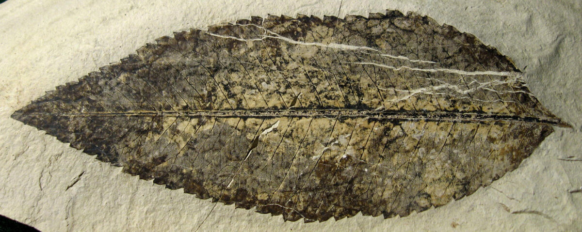
Feature image: The fossil leaf Photonia pagae, a toothed leaf from the Eocene Republic flora of Washington, U.S.A. Photo by Kevmin (Wikimedia Commons, Creative Commons Attribution-ShareAlike 3.0 Unported license, image cropped and resized)
Introduction
Leaf margin analysis (LMA) is a method that uses one leaf characteristic, the margin (edge), to estimate mean annual temperature (MAT, meaning average yearly temperature).
LMA is based upon the observation that woody dicots (generally speaking, broadleaved trees and shrubs) that have leaves with entire margins usually make up a greater proportion of the flora in warmer climates than in cooler climates. In the strict sense, a leaf with an entire margin has an edge that is smooth. In modern LMA analyses, species with lobed leaves are categorized as entire if they do not have teeth. Thus, the "entire" category is sometimes called untoothed, which is a more accurate descriptor.
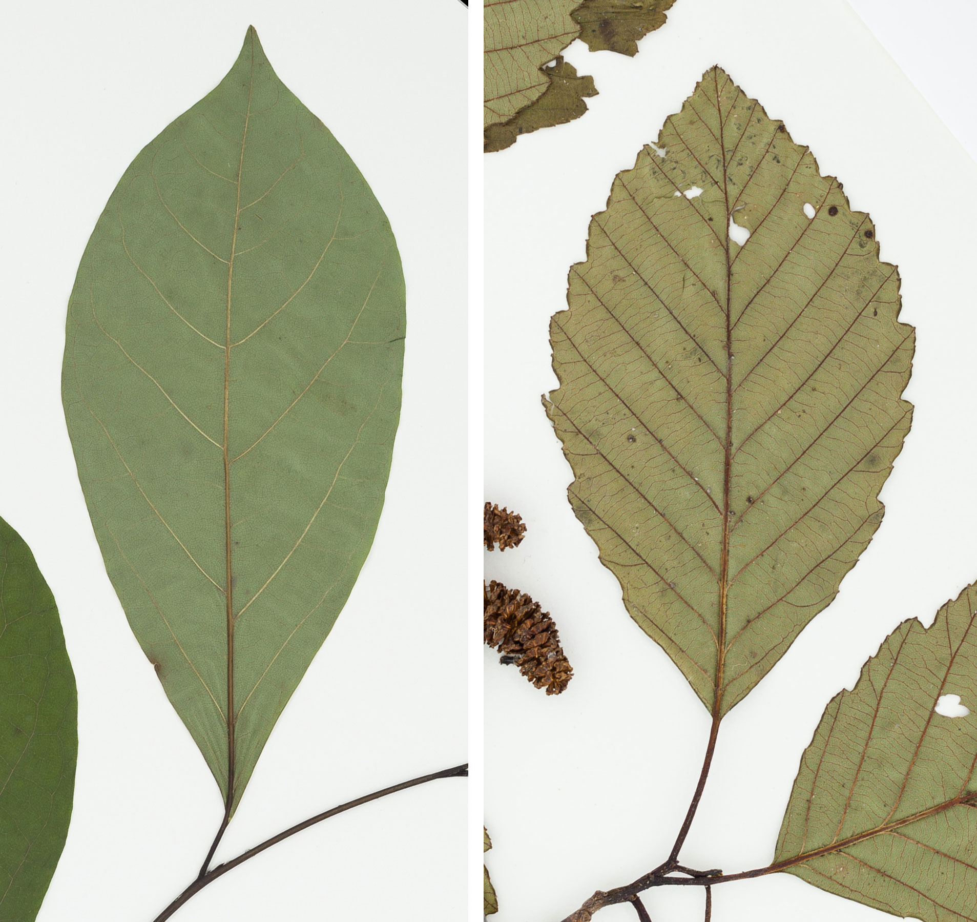
Unlobed untoothed (left) and toothed (right) leaves. Left: A leaf of northern spicebush (Lindera benozoin) without teeth. Right: A leaf of red alder (Alnus rubra) with teeth. Credits: Lindera benzoin, NY 02549603 and Alnus rubra, NY02472467 (both images by New York Botanical Garden, via GBIF, CC BY 4.0, images rotated and cropped).
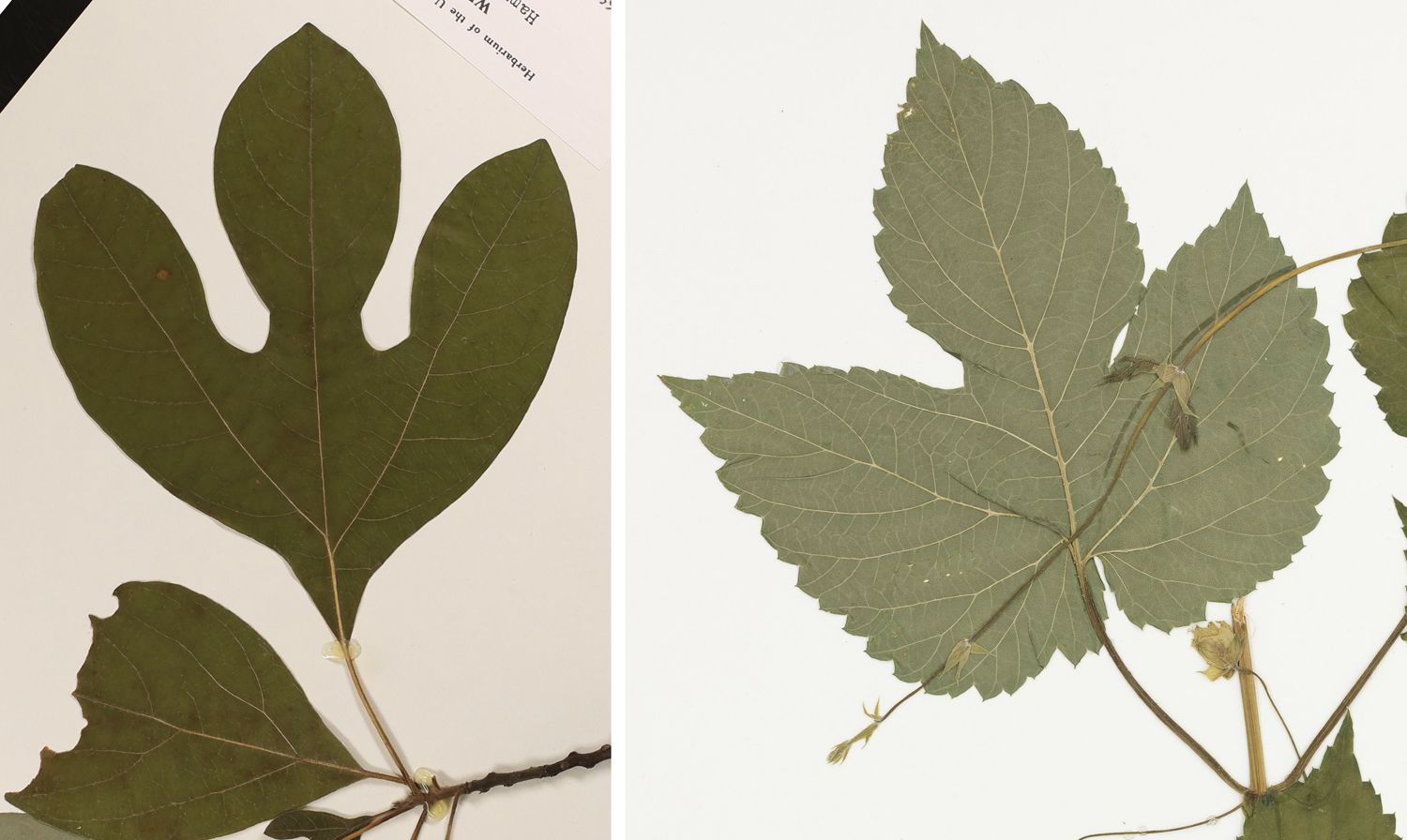
Lobed untoothed (left) and toothed (right) leaves. Left: A three-lobed leaf of sassafras (Sassafras albidum) without teeth (the tip of the left leaf lobe is broken off). Right: A three-lobed leaf of hops (Humulus lupulus) with teeth. Credits: Sassafras albidum, NCU00314272 (University of North Carolina at Chapel Hill Herbarium, via GBIF, CC BY-NC 3.0); Humulus lupulus, NY3883733 (New York Botanical Garden, via GBIF, CC BY 4.0).
Scoring leaves for LMA
To begin calculating mean annual temperature (MAT) using LMA, the total number of woody dicot species (or morphotypes) in a flora must be determined, as well as the number of woody dicot species with untoothed leaves. The number of species with untoothed leaves added to the number of species with toothed leaves should equal the total number of species in a flora. If a particular plant species has both toothed and untoothed leaves, it is counted as half a species (0.5) in each category.
Example table for tabulating the numbers of species (or morphotypes) with untoothed and toothed leaves in a flora
| Species or morphotype | Untoothed | Toothed | Total species or morphotypes |
|---|---|---|---|
| Species A | 1 | 0 | |
| Species B | 0 | 1 | |
| Species C | 0 | 1 | |
| Species D | 0.5 | 0.5 | |
| Species E | 1 | 0 | |
| Total | 2.5 | 2.5 | 5 |
In the table above, the flora has a total of five species or leaf morphotypes. Two species (A and E) have untoothed leaves, two species (B and C) have toothed leaves, and one species (D) has both untoothed and toothed leaves. Thus, each category (untoothed and toothed) has a total of 2.5 species or morphotypes.
LMA equations use the percent (E) of species or morphotypes with untoothed leaves to calculate MAT. In order to calculate the percent, divide the number of species or morphotypes with untoothed leaves by the total number of species or morphotypes, then multiple by 100.
E = number of species or morphotypes with untoothed leaves ÷ total number of species or morphotypes × 100
In the example above:
E = 2.5 ÷ 5 × 100 = 50%
Origin of LMA
LMA is rooted in observations published by Irving W. Bailey and Edmund W. Sinnott in the early 1900s. These researchers showed that the warmer the climate, the more woody dicot species with entire-margined leaves were present in the flora; as a corollary, colder climates have more woody dicot species with toothed leaves.
There are some exceptions to this rule. For example, the association between colder climate and toothed leaves breaks down in very cold and dry environments, which also have a higher percentage of entire-margined species.
Bailey and Sinnott later applied their data from modern plants to fossil floras. They calculated the percent entire-margined species for some Cretaceous and Cenozoic floras. They compared the values from the fossil floras to those of modern floras to provide a rough interpretation of the environments represented by the fossil floras.
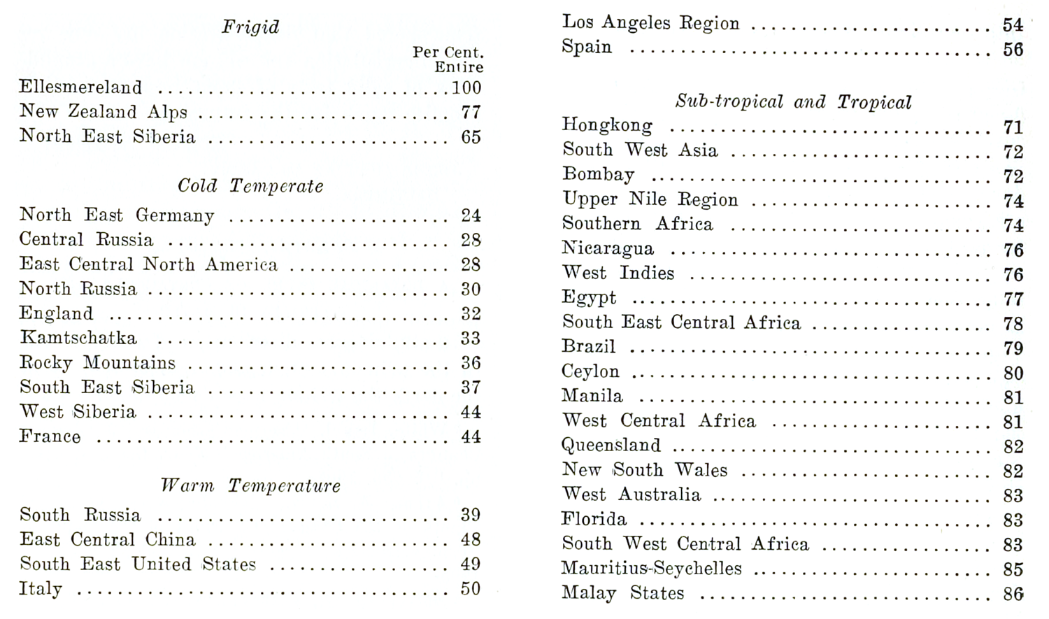
Percent entire-margined woody dicot species in modern floras from Bailey & Sinnott (1915). The table above shows the percent entire-margined woody dicot species in global floras, separated into broad categories. Note that as climate gets warmer, the percent entire-margined species increases, moving from cold temperate (24%–44% entire-margined species), to warm temperate (39%–56% entire-margined species), to subtropical/tropical (71%–86% entire-margined species). Frigid floras (65%–100% entire-margined species) do not follow this trend. Credit: Reproduced from Bailey & Sinnott (1915) Science 41: pg. 832 (via Biodiversity Heritage Library, Public Domain). Image modified from original.
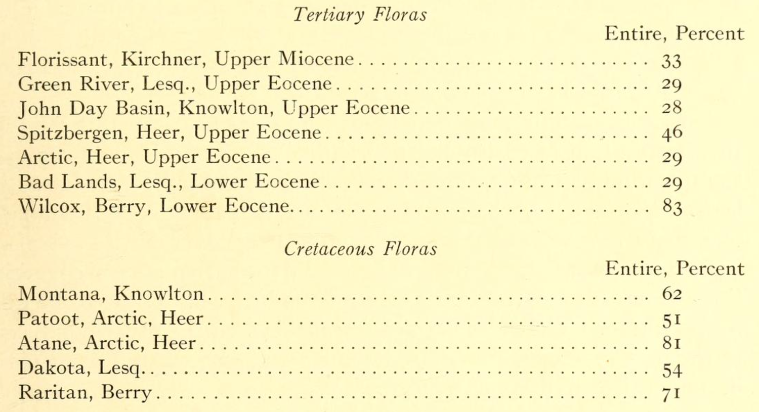
Percent entire-margined wood dicot species from fossil floras from Bailey & Sinnott (1916). This table shows the percent entire-margined woody dicot species from fossil floras in the Cretaceous and Tertiary (mostly Paleogene; note that Florissant is now considered to be late Eocene in age). Cretaceous floras range from 62%–71%, Tertiary floras from 28%–83%. Credit: Reproduced from Bailey & Sinnott (1916) Amer J Bot 3: pg. 37, table 6 (via Biodiversity Heritage Library, Public Domain).
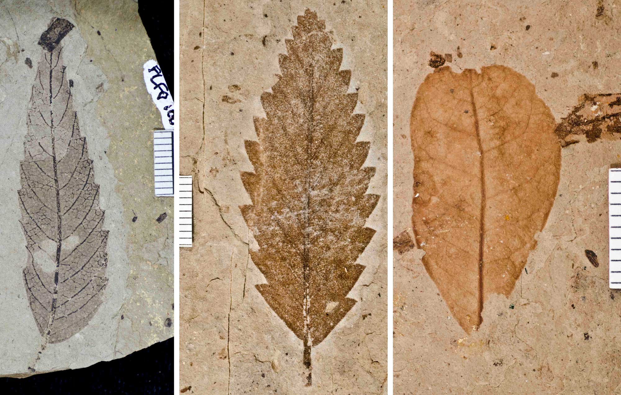
Leaves from the Eocene Florissant flora of Colorado. The Florissant flora is dominated by species (or morphotypes) with toothed leaves. From left to right, these leaves are from an extinct member of the elm family (Cedrelospermum, toothed), an extinct member of the beech family (Fagopsis, toothed), and a smoketree (Cotinus, untoothed). All photos by National Park Service/NPS (public domain).
LMA equations
The original LMA equation
Wolfe (1993) graphed the correlation between higher mean annual temperature (MAT) and more entire-margined species using data from East Asian floras. Using Wolfe's data, Wing and Greenwood (1993) later developed an equation to calculate MAT from the percent of woody dicot species with entire-margined leaves in a flora. Their equation is:
MAT = (0.306 × percent entire-margined species) + 1.141
This equation is based on the slope-intercept equation for a line. So, where does the line that defines this equation come from? It comes from making a graph of data from modern floras.
For the equation above, data from East Asian floras were plotted. As in the graph below, the percent of entire-margined species for each flora was plotted on the x-axis, and the corresponding mean annual temperature for each flora was plotted on the y-axis. Then, the best-fitting regression line was drawn through the data points. (Regression lines can be calculated by hand or, more conveniently, by a computer.)
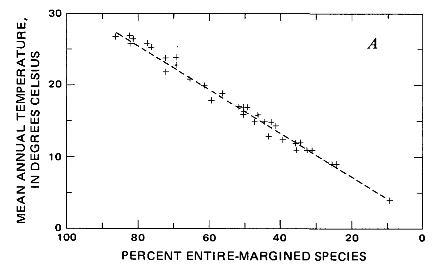
Correlation between leaf margin and MAT for East Asian forests. This graph, compiled by J.A. Wolfe, is based on "local floras in the humid to mesic forests of eastern Asia." The plus-signs are data points. The dotted line is a regression line that has been fitted to the data. Credit: Reproduced from Wolfe (1979) USGS Professional Paper 1106: pg. 35, fig. 8a.
The general slope-intercept equation describing a line is:
y = mx + b
Where:
y = the y coordinate.
In the LMA equation above, y is the mean annual temperature (MAT). MAT is the value being calculated.
x = the x coordinate.
In the LMA equation above, x is the percent entire-margined woody dicot species in a given flora. [Percent entire-margined woody dicot species = (number of entire-margined woody dicot species ÷ total number of woody dicot species) × 100]
m = the slope of the line. Slope = (change in y) ÷ (change in x).
In the LMA equation above, this value is 0.306. A slope of 0.306 means that for every 0.306°C change in mean annual temperature (MAT or y), there is a 1% change in the percent of entire-margined woody dicot species in a flora (x). Also, temperature and percent entire-margined species are positively correlated, so as one increases, so does the other.
b = the y-intercept. In other words, when x = 0, what is y?
In the LMA equation above, this value is 1.141. Remember, x in this equation is percent entire-margined woody dicot species, so the y-intercept is the predicted MAT (1.141°C) when there are no entire-margined woody dicot species in a flora. (In the graph above, the y-intercept is on the right-hand side.)
Wing and Greenwood (1993) used their equation to estimate the MAT for several North American fossil leaf floras. In order to do this, all they needed to figure out was the percent of woody dicot species with entire-margined leaves in each flora. For example, in the Eocene Wind River flora from Wyoming, they calculated that 57% of woody dicot species had leaves with entire margins. Using their equation:
MAT = 0.306 × 57 + 1.141 = 18.6°C
In the Eocene Green River (Parachute Creek Member or Lake Uinta) flora of Colorado and Utah, they calculated that 46% of woody dicot species had leaves with entire margins. Again, using their equation:
MAT = 0.306 × 46 + 1.141 = 15.2°C
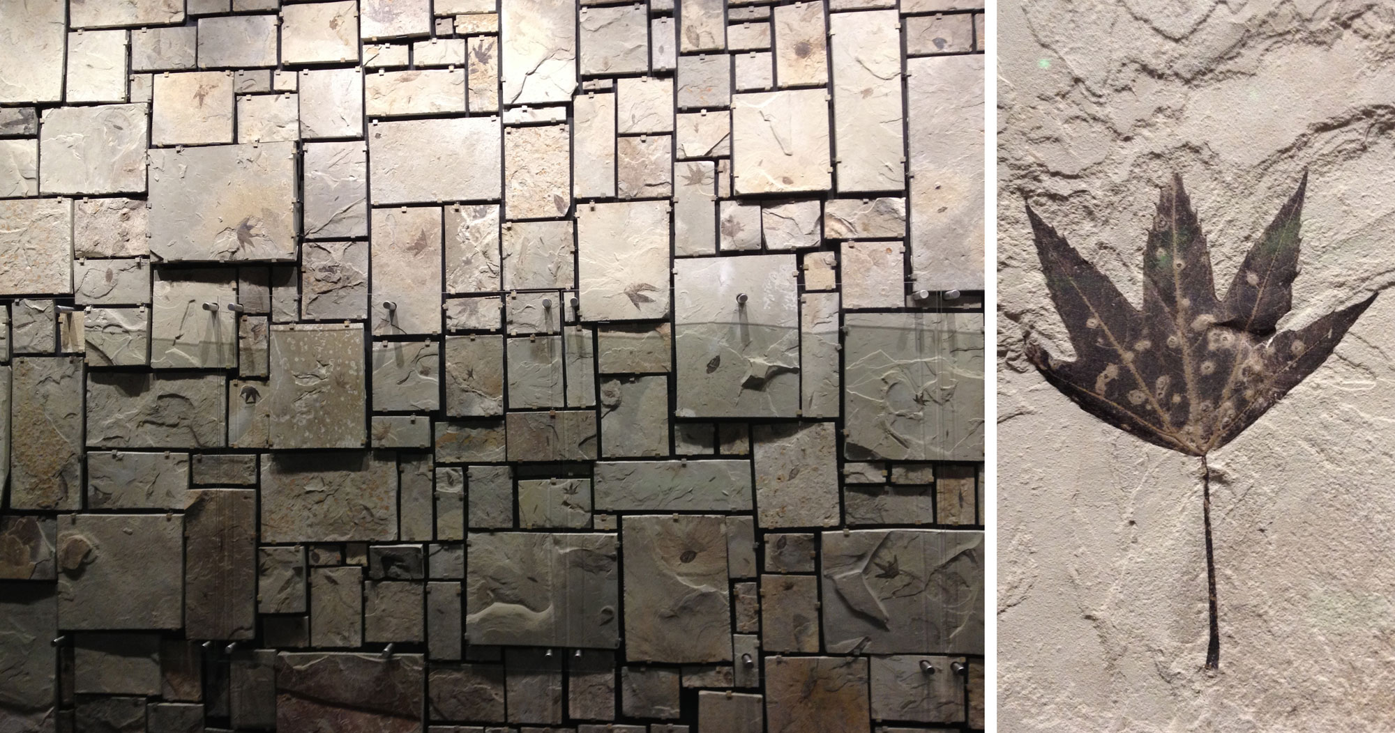
Eocene Green River Formation (Parachute Creek Member) plant fossils at display at the Utah State Field House of Natural History in Vernal, Utah. Left: Wall of plant fossils. Right: Specimen of Macginitea, an extinct relative of the modern sycamore (Platanus). Photos by Jonathan R. Hendricks (2014), originally published on Earth@Home (Creative Commons Attribution-NonCommercial-ShareAlike 4.0 International license).
Other LMA equations
Data from the forests of eastern Asia cannot necessarily be applied to floras from other regions of the world. Differences in the percent of woody dicot species with entire-margined leaves between regions may be caused by the differing phylogenetic make-up of regional floras; in other words, different plant lineages dominate different regions of the world and may respond somewhat differently to changes in mean annual temperature.
Since the first LMA equation was published, many other LMA formulas have been proposed. These equations are based on regional floras from different parts of the world and take the following general form:
MAT = mE + b
Where:
MAT = leaf mean annual temperature, the value that is being calculated.
m = the slope of the line. The slope varies from formula to formula.
E = percent entire-margined (meaning untoothed) woody dicot leaf species or morphotypes.
b = the y-intercept. This value varies depending on the equation.
Sometimes, the y-intercept is negative, in which case the equation is:
MAT = mE − b
Peppe et al. (2018) developed a global LMA equation by combining data from different major regions of the world. That equation is:
MAT = 0.194E + 5.884
Variations in the way the LMA equation is written
It should be noted that there are sometimes variations in the way the LMA equation is presented. Another common way to write the general LMA equation is:
LMAT = (100m)P + b
Where:
LMAT = Leaf-estimated mean annual temperature, indicating that the mean annual temperature is calculated from leaves.
100m = The slope multiplied by 100.
P = Fraction of species or morphotypes with entire-margined leaves expressed as a decimal. [Fraction of entire-margined woody dicot species or morphotypes = number of entire-margined woody dicot species or morphotypes ÷ total number of woody dicot species or morphotypes.]
b = the y-intercept.
Using this format, the Peppe et al. (2018) global equation can also be written as:
LMAT = 19.4P + 5.884
Notice that this equation and the one provided in the preceding section will yield the same result.
Why do toothed leaves occur in cooler climates?
Of course, all of the discussion above prompts the question: Why are toothed leaves associated with cooler climates? This is still an area of active research, and scientists have proposed various ideas. Notably, toothed leaf margins co-occur with other features—like seasonal shedding of leaves (deciduousness) and thinner leaves—that also tend to characterize woody plants in cooler climates. One of the more likely explanations for the correlation between toothed leaves and cooler climates is physiological. Namely, teeth are areas of active photosynthesis in the spring, when seasonal growth first begins.
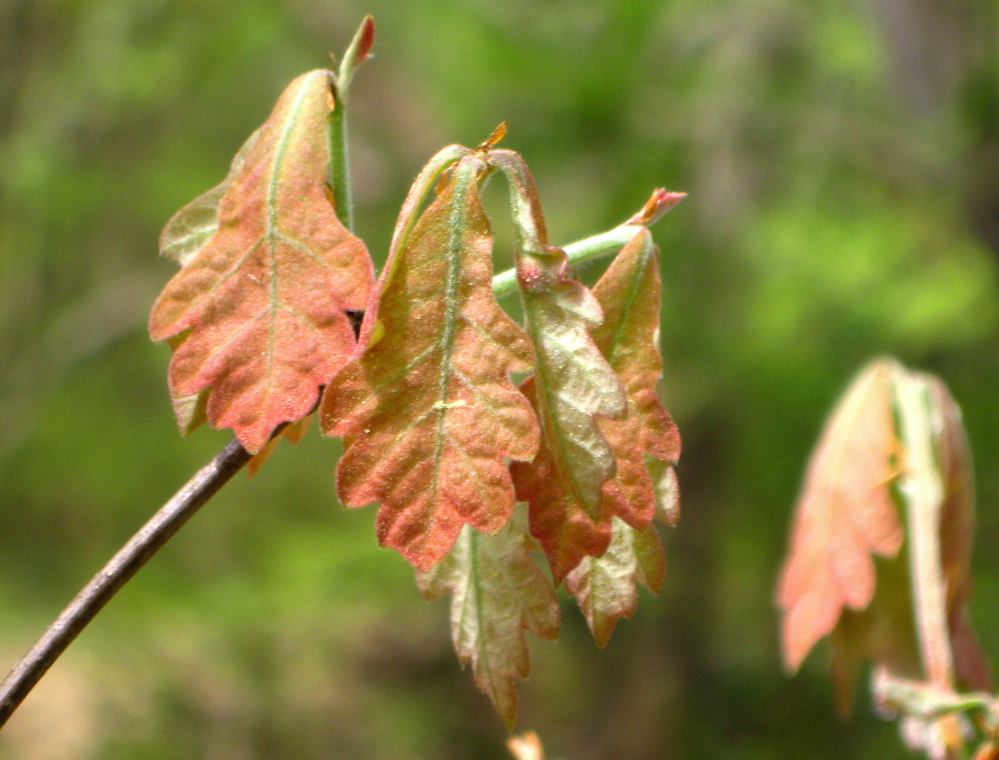
Spring growth of white oak (Quercus alba) leaves. Photo "New white oak leaves" by Matt Jones (NatureServe on flickr, CC BY 2.0, image cropped and resized).
Error & accuracy
Leaf margin analysis has a few things going for it as a method. LMA relies on only one type of observation and a simple equation to calculate. Observing whether leaves are toothed or untoothed is relatively straightforward and objective compared to observing and scoring some other leaf characteristics that have been used in paleoclimate reconstruction. Also, the correlation between untoothed leaves and warmer climate appears to be robust, and LMA estimates appear to be reasonably accurate.
Most equations for LMA have a suggested standard error expressed as ± XºC. One debate regarding LMA is how to calculate the error associated with MAT estimates from LMA equations. Specifically, some methods of calculating the error appear to overestimate the precision of the method (in other words, they suggest an error that is too small). For their global LMA equation, Peppe et al. (2018), reported that the minimum error is ± 4.54°C.
References & further reading
Note: Free full text is made available by the publisher for items marked with a green asterisk.
Academic articles & book chapters
Bailey, I.W., and E.W. Sinnot. 1915. A botanical index of Cretaceous and Tertiary climates. Science 41: 831–834. https://doi.org/10.1126/science.41.1066.831. Read/download free on Biodiversity Heritage Library: https://www.biodiversitylibrary.org/bibliography/44793#/summary
Bailey, I.W., and E.W. Sinnott. 1916. The climatic distribution of certain types of angiosperm leaves. American Journal of Botany 3: 24–39. Read/download free on Biodiversity Heritage Library: https://www.biodiversitylibrary.org/bibliography/101582#/summary
* Peppe, D.J., A. Baumgartner, A. Flynn, and B. Blonder. 2017. Reconstructing paleoclimate and paleoecology using fossil leaves, ver. 2. PaleorXiv. [Preprint] https://doi.org/10.31233/osf.io/stzuc
Peppe, D.J., A. Baumgartner, A. Flynn, and B. Blonder. 2018. Reconstructing paleoclimate and paleoecology using fossil leaves. Pp. 289–317 in D.A. Croft, D.F. Su, and S.W. Simpson, eds. Methods in Paleoecology: Reconstructing Cenozoic Terrestrial Environments. Springer Nature Switzerland AG, Switzerland. https://doi.org/10.1007/978-3-319-94265-0_13
Royer, D.L., and P. Wilf. 2005. Why do toothed leaves correlate with cold climates? Gas exchange at leaf margins provides new insights into a classic paleotemperature proxy. International Journal of Plant Sciences 167: 113–118. https://doi.org/10.1086/497995
* Royer, D.L., D.J. Peppe, E.A. Wheeler, and Ülo Niinemets. 2012. Roles of climate and functional traits in controlling toothed vs. untoothed leaf margins. American Journal of Botany 99: 915–922. https://doi.org/10.3732/ajb.1100428
* Seyfullah, L.J. 2012. Fossil focus: Using plant fossils to understand past climates and environments. Palaeontology [Online] 2(7): 1–8. https://www.palaeontologyonline.com/articles/2012/fossil-focus-plant-fossils/
Wilf, P. 1997. When are leaves good thermometers? A new case for Leaf Margin Analysis. Paleobiology 23: 373–390. https://doi.org/10.1017/S0094837300019746
Wing, S.L., and D.R.Greenwood. 1993. Fossils and fossil climate: The case for equable continental interiors in the Eocene. Philosophical Transactions: Biological Sciences 341: 243–252. https://doi.org/10.1098/rstb.1993.0109
* Wolfe, J.A. 1979. Temperature parameters of humid to mesic forests of eastern Asia and relation to forests of other regions of the Northern Hemisphere and Australasia. United States Geological Survey Professional Paper 1106, 37 pgs. https://doi.org/10.3133/pp1106
Websites
Research part 2: Leaf Margin Analysis (UWYO Dioramas): https://uwyodioramas.wordpress.com/2013/02/26/research-and-leaf-margin-analysis/
Content usage
Usage of text and images created for DEAL: Text on this page was written by Elizabeth J. Hermsen. Original written content created by E.J. Hermsen for the Digital Encyclopedia of Ancient Life that appears on this page is licensed under a Creative Commons Attribution-NonCommercial-ShareAlike 4.0 International License. Original images created by E.J. Hermsen are also licensed under Creative Commons Attribution-NonCommercial-ShareAlike 4.0 International License.
Content sourced from other websites: Attribution, source webpage, and licensing information or terms of use are indicated for images sourced from other websites in the figure caption below the relevant image. See original sources for further details. Attribution and source webpage are indicated for embedded videos. See original sources for terms of use. Reproduction of an image or video on this page does not imply endorsement by the author, creator, source website, publisher, and/or copyright holder.
Adapted images. Images that have been adapted or remixed for DEAL (e.g., labelled images, multipanel figures) are governed by the terms of the original image license(s) covering attribution, general reuse, and commercial reuse. DEAL places no further restrictions above or beyond those of the original creator(s) and/or copyright holder(s) on adapted images, although we ask that you credit DEAL if reusing an adapted image from the DEAL website. Please note that some DEAL figures may only be reused with permission of the creator(s) or copyright holder(s) of the original images. Consult the individual image credits for further details.
Last updated 28 July 2022.